Classification and Clustering of Mice
Statement of Overall Problem
The mouse style research investigates mouse behaviors of different genes. The researchers hope to gain insight to human behaviors using mouse data, since experimenting directly on human is difficult.
The important concern is whether we can classify different strains of mice based on mouse behaviors through machine learning algorithms. Important features in classification models will be extracted for future study. The fundamental hypothesis is that different mouse strains have different behaviors, and we are able to use these behaviors as features to classify mice successfully. On the other hand, we are also trying to use unsupervised clustering algorithms to cluster mice, and ideally different strains should have different clustering distributions.
Statement of Statistical Problems
The researchers design the experiment as follows: they have 16 different strains of mice, and each strain has 9 to 12 almost identical male mice in terms of genes.
We first need to verify the assumption that mouse of different strains do exhibit different behaviors. One way to do this is to perform hypothesis testing based on the joint distribution of all the features. A simpler alternative is to perform EDA on each of the features. If we observe that each mouse behaves very similarly to its twins, but differently from other strains of mice, we can conclude that genetic differences affect mouse behaviors and that behavioral features might be important for classification. Notice that here we can evaluate the difference by assessing the classification performance of models based on behavioral features.
Classification
Based on the assumption, the problem is inherently a multiclass classification problem based on behavioral features either directly obtained during the experiment or artificially constructed. Here we have to determine the feature space both from the exploratory analysis and biological knowledge. If the classification models performed well, we may conclude that behavioral differences indeed reveal genetic differences, and dig into the most important features needed seeking the biological explanations. Otherwise, say if the model fails to distinguish two different strains of mice, we may study that whether those strains of mice are genetically similar or the behavior features we selected are actually homogeneous through different strains of mice.
Clustering
To extend the scope of the analysis, the clustering analysis may also be used to analyze mouse behaviors. Though these mice had inherent strain labels, the clusters may not follow the strain labels because genetical differences are not fully capturing the behavioral differences. Moreover, determining the best number of clusters is key in assessing the performance of a clustering model. Notice that the best number of clusters are neither necessarily equal to 16 nor the same across different clustering methods. Criterion like silhouette scores would be evaluated to choose the best number of clusters. Petkov’s paper also give us ideas about clustering and the difference between each strains [PDC+04].
Exploratory Analysis & Classification Models
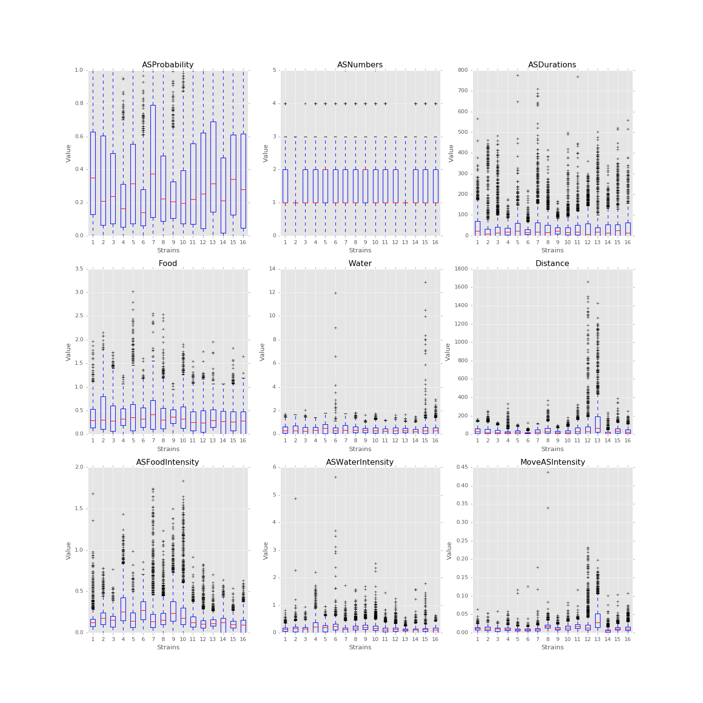
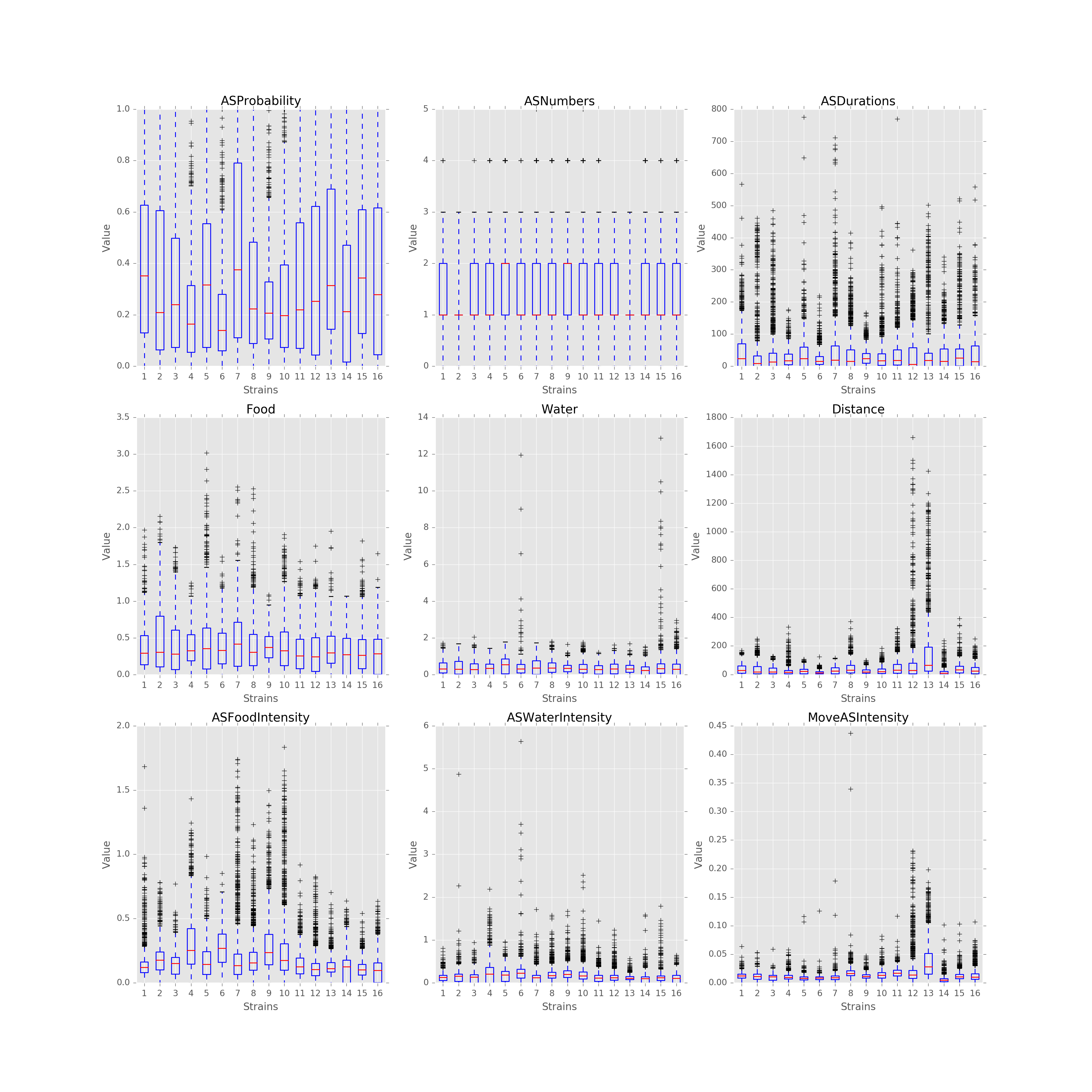
In 1D, box plots of each feature, say food consumption or sleeping time, of each strain are plotted below. In 2D, PCA can be performed on the feature data set and the data are then plotted along the first and the second principal axes colored in different strains. These plots are useful in verifying assumptions. For instance, we could box-plot different strains of mice against food consumption to see whether different strains of mice eat distinctly. If the number of variables needed to be evaluated is large, we might also use five number summaries to study the distributions.
(Source code, png, hires.png, pdf)

Boxplots of the features over 170 mice
Since each strain (each class) only has 9 to 12 mice, inputting too many features to the classification model is unwise. The exploratory data analysis will be an important step for hypothesis testing and feature selection. The process will also help us to find outliers and missing values in each behavioral variable, and we will decide how to handle those values after encountering that.
Data Requirements Description
For this project, we use behavioral data recorded for each mouse and each two-hour time bin of the day. There are in total 170 mice across 16 different strains. Behavioral features include measurements of daily activities, such as food and water consumption, distance moved, the amount of time a mouse is in active state, and the amount of time a mouse spends eating, drinking and moving while in active state.
For classification and clustering subsections, we require different processed data.
For classification project, we have two different datasets – mouseday dataset or individual mouse dataset. For the mouseday dataset, we take each combination of mouse and day as a unique observation, resulting in 1921 observations. For the individual mouse dataset, we take the average measures of different days for each mouse to form 170 unique observations. In each dataset, we use the measures for different time bins as different features. Therefore, we have a maximum of 9 types of features * 11 time bins = 99 features. Users can also use a subset of these 99 features to train models. The mouse strain number will serve as the label for the dataset.
For clustering project, we used the individual mouse dataset which has 170 observations. For clustering, we do not want too many features since these features might have directions very close to each other and it would be repetitive to use all of them. Therefore, instead taking each hour bin as different features like in the classification dataset, we take each hour bin as different observations, resulting in only 9 features for the clustering data. Then we take average of days for each mouse. While preparing the input data, users will also have the choice to standardize data and/or add the standard deviation for each of the 9 features, resulting in possibly 18 final features. One thing to note is that we did not use mouseday data to perform clustering, although it is possible to do with our function. The reason we are not using big dataset is because the hierarchical clustering is computationally expensive and silhouette score also takes fairly long time to calculate.
Methodology
Classification
For this project, we mainly focus on three classification algorithms, which are random forests, gradient boosting and support vector machines (SVM).
Introduction
Random forests is a notion of the general technique of random decision forests that are an ensemble learning method for classification, regression and other tasks, that operate by constructing a multitude of decision trees at training time and outputting the class that is the mode of the classes (classification) of the individual trees. The method combines Breiman’s “bagging” idea and the random selection of features, correcting for decision trees’ habit of overfitting to their training set.
Gradient boosting is another machine learning algorithm for classification. It produces a prediction model in the form of an ensemble of weak prediction models, typically decision trees. Gradient boosting fits an additive model in a forward stage-wise manner. In each stage, it introduces a weak learner to compensate the shortcomings of existing weak learners, which allows optimization of an arbitrary differentiable loss function.
Support vector Machines (SVM) are set of related supervised learning methods for classification and regression, which minimize the empirical classification error and maximize the geometric margin. SVMs map the input vector into a higher dimensional space where the maximal separating hyper plane is constructed. By maximizing the distance between different parallel hyper planes, SVMs come up with the classification of the input vector.
Tuning Parameters
For each of the algorithms, we create functions to fit them on the dataset. There are two different ways to fit these methods: if the user pre-defines the set of the parameters, we will use cross validation to find the best estimators and their relative labels; if the user does not define the parameters, the functions will use the default values to fit the models.
For random forests, we tune n_estimators, max_feature and importance_level. n_estimators represents the number of trees in the forest. The larger, the more accurate. However, it takes considerable amount of computational time when increasing forest size. max_features represents the number of features to consider when looking for the best split. max_depth represents the maximum depth of the tree. The larger, the more accurate. However, it takes considerable amount of computational time when increasing tree size.
For gradient boosting, we tune n_estimators and learning_rate. n_estimators represent the number of boosting stages to perform. Gradient boosting is fairly robust to over-fitting, therefore, a larger number represents more performing stages, usually leading to better performance. learning_rate will shrink the contribution of each tree by the value of learning_rate. There is a trade-off between learning_rate and n_estimators. We use GridSearch to tune the learning_rate in order to find the best estimator.
For SVM, we tune C and gamma. C represents the penalty parameter of the error term. It trades off misclassification of training examples against simplicity of the decision surface. A low C makes the decision surface smooth, while a high C aims at classifying all training examples correctly. Gamma is the Kernel coefficient for ‘rbf’, ‘poly’ and ‘sigmoid’. It defines how far the influence of a single training example reaches, with low values meaning ‘far’ and high values meaning ‘close’.
Model Assessment
After tuning our parameters, we apply our models to testing set and compare the prediction labels with the true labels. There are two major ways to measure the quality of the prediction process, one is a confusion matrix and the other is percentage indicators including precision, recall, and F-1 measure. A confusion matrix is a specific table layout that allows visualization of the performance of an algorithm. Each row of the matrix represents the instances in a predicted class while each column represents the instances in an actual class. The name stems from the fact that it makes it easy to see if the system is confusing two classes (i.e. commonly mislabeling one as another).
precision(P) = \(\frac{\# label\ y\ \ predicted\ correctly}{\# label\ y\ predicted}\)
recall(R) = \(\frac{\# label\ y\ \ predicted\ correctly}{\# label\ y\ true}\)
F-1 = \(\frac{2*P*R}{P+R}\)
Thus, precision for each label is the corresponding diagonal value divided by row total in the confusion matrix and recall is the diagonal value divided by column total.
Clustering
Unsupervised learning clustering algorithms, K-means and hierarchical clustering, are included in the subpackage classification. Unlike other clustering problems where no ground truth is available, the biological information of the mice allows us to group the 16 strains into 6 larger mouse families, although the ‘distances’ among the families are unknown and may not be comparable at all. Hence, cluster numbers from 2 to 16 should all be tried out to find the optimal. Here, we briefly describe the two algorithms and the usage of the related functions.
Above all, note that unlike the supervised classification problem where we have 11 levels for one feature (so we have up to 99 features in the classification problem), the unsupervised clustering methods could suffer from curse of high dimensionality when we input a large amount of features. In high dimension, every data point is far away from each other, and the useful feature may fail to stand out. Thus we decided to use the average amount of features over a day and the standard deviation of those features for the individual mouse (170 data points) case.
K-means
To begin with, K-means minimizes the within-cluster sum of squares to search for the best clusters set. Then the best number of clusters was determined by a compromise between the silhouette score and the interpretability. K-means is computationally inexpensive so we can either do the individual mouse options (170 data points). However, the nature of K-means makes it perform poorly when we have imbalanced clusters.
Hierarchical Clustering
Given the above, the potentially uneven cluster sizes lead us to consider an additional clustering algorithm, hierarchical clustering, the functionality of which is included in the subpackage. Generally, hierarchical clustering seeks to build a hierarchy of clusters and falls into two types: agglomerative and divisive. The agglomerative approach has a “richer get richer” behavior and hence is adopted, which works in a bottom-up manner such that each observation starts in its own cluster, and pairs of clusters are merged as one moves up the hierarchy. The merges are determined in a greedy manner in the sense that the merge resulting in the greatest reduction in the total distances is chosen at each step. The results of hierarchical clustering are usually presented in a dendrogram, and thereby one may choose the cutoff to decide the optimal number of clusters.
Below is a demo to fit the clustering algorithm. The loaded data is firstly standardized, and then the optimal distance measure and the optimal linkage method are determined. We have restricted the distance measure to be l1-norm (Manhattan distance), l2-norm (Euclidean distance) and infinity-norm (maximum distance), and the linkage method to be ward linkage, maximum linkage and average linkage. The maximum linkage assigns the maximum distance between any pair of points from two clusters to be the distance between the clusters, while the average linkage assigns the average. The ward linkage uses the Ward variance minimization criterion. Then, the optimal linkage method and distance measure are input to the model fitting function, and the resulting clusters and corresponding silhouette scores are recorded for cluster number determination. A plotting function from the subpackage is also called to output a plot. The output plot is included in the result section of the report.
from mousestyles import data
from mousestyles.classification import clustering
from mousestyles.visualization import plot_clustering

# load data
mouse_data = data.load_all_features()

# rescaled mouse data
mouse_dayavgstd_rsl = clustering.prep_data(
mouse_data, melted=False, std=True, rescale=True)

# get optimal parameters
method, dist = clustering.get_optimal_hc_params(mouse_day=mouse_dayavgstd_rsl)

# fit hc
sils_hc, labels_hc = clustering.fit_hc(
    mouse_day_X=mouse_dayavgstd_rsl[:,2:],
    method=method, dist=dist, num_clusters=range(2,17))

# plot
plot_clustering.plot_dendrogram(
    mouse_day=mouse_dayavgstd_rsl, method=method, dist=dist)
Testing Framework Outline
To ensure our functions do the correct steps and return appropriate results, we also implemented test functions. For clustering, we first perform basic testing of whether our output has appropriate number of values or values we expect. One more advanced check we perform is to test whether we successfully assign cluster numbers to every observation. Also, since we compute silhouette score for each cluster and silhouette score is defined to be between -1 and 1, we also checked that whether our silhouette score is appropriate. For classification, we also checked whether our final predictions of mouse strains only include numbers 0 through 15 since they are the only strains for data we have and we should predict those strains.
Result
Classification
For three models, after tuning the parameters and output the prediction result, we create the side-by-side barplot for the different measurement of accuracy, which are precision, recall and F1.
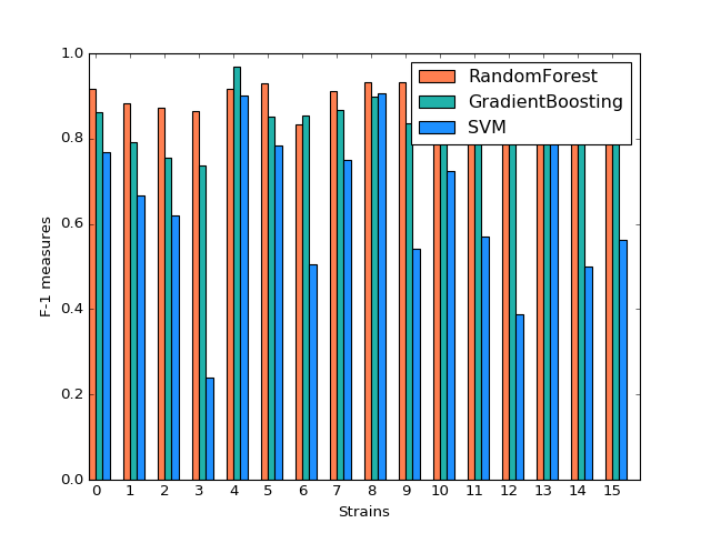
Random Forest
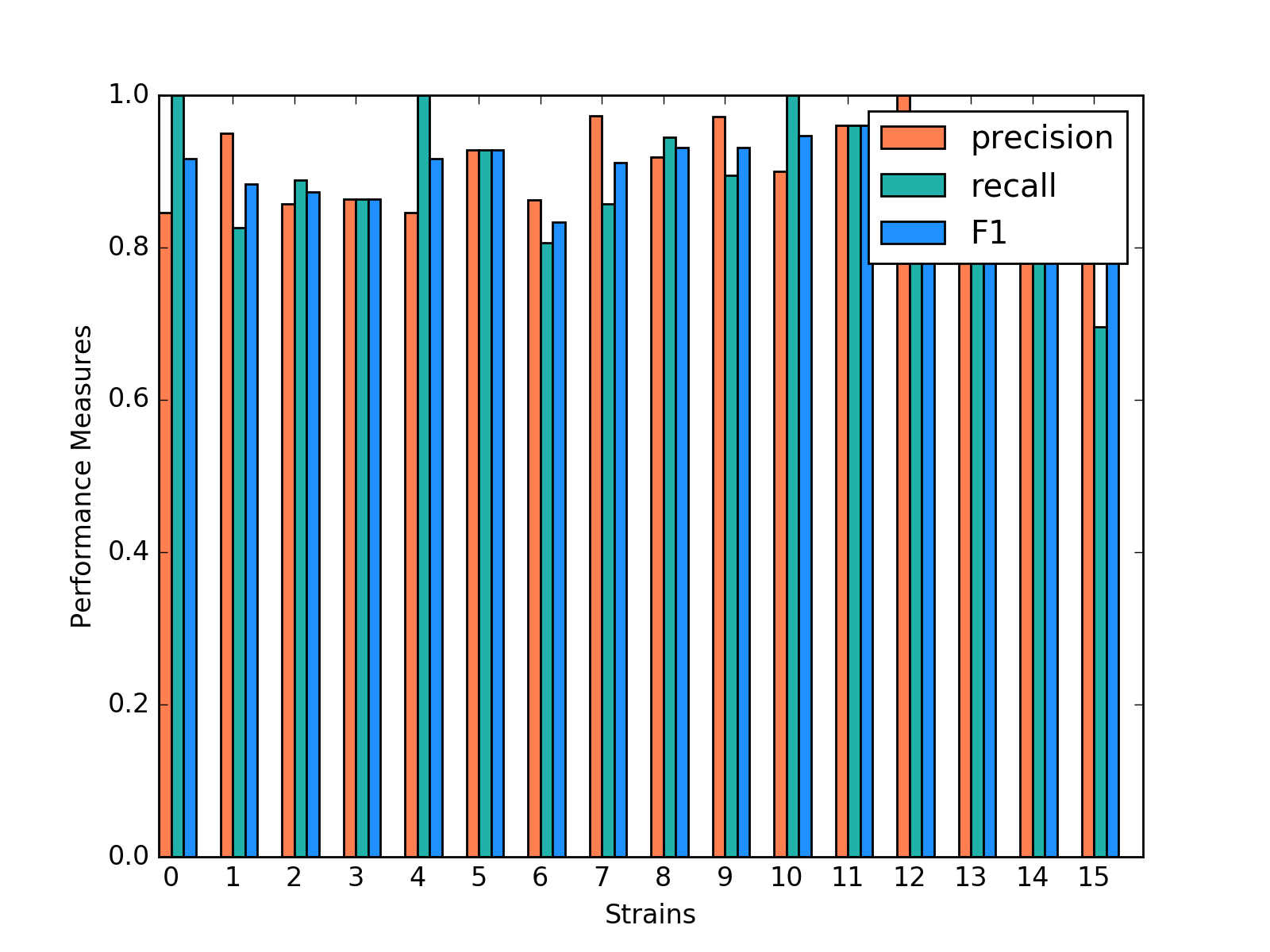
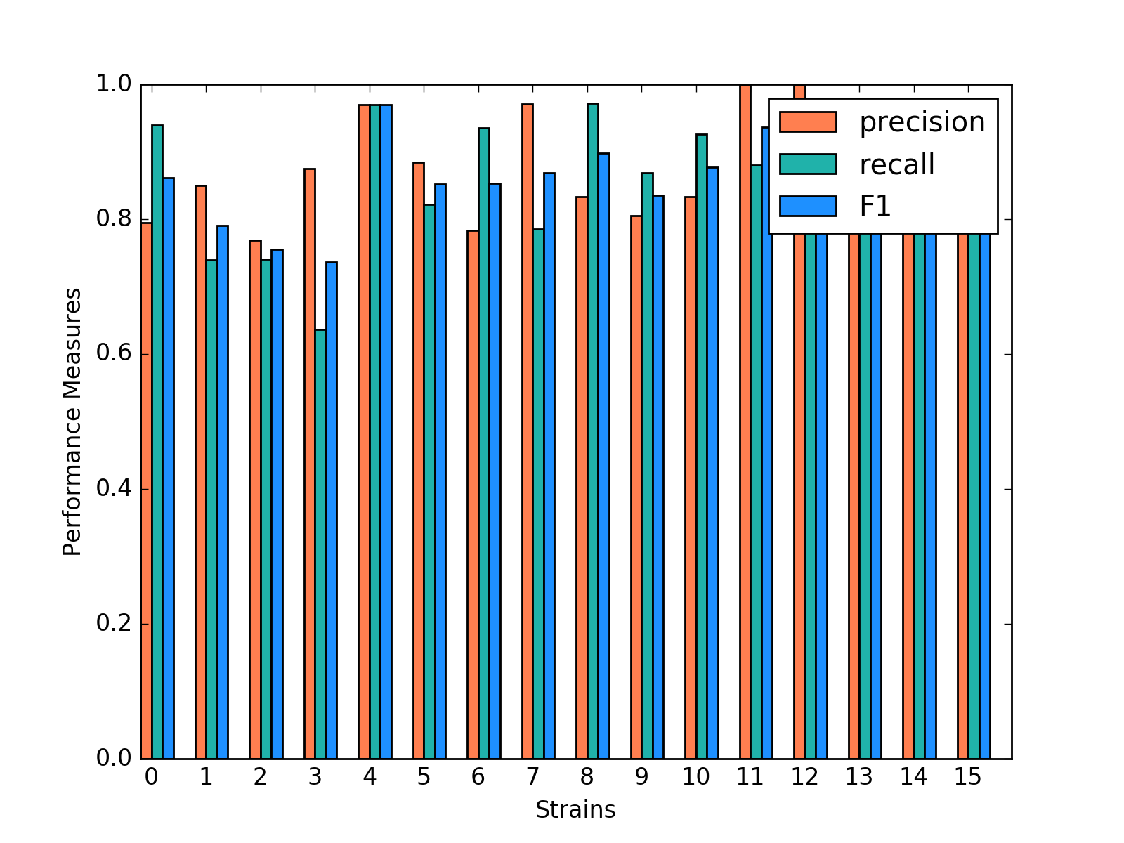
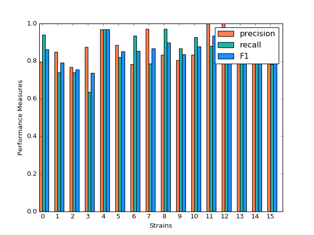
Random Forest shows a very promising result. For each strain, prediction, recall and F-1 measure are very close to each other. Except for predicting strain 15, all the other prediction has F-1 measure exceeding 0.8.
(Source code, png, hires.png, pdf)
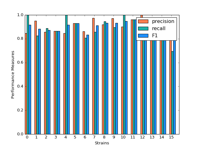
Classification Performance of Random Forest
We also select the most important features, including ASProbability_2, Distance_14, ASProbability_16, Distance_2, Food_4, MoveASIntensity_2, ASProbability_4, Distance_4, Distance_16.
Gradient Boosting
Gradient Boosting shows a decent performance on the prediction. There is no huge difference in precision and recall for predicting each strain, but bigger than Random Forest. It is shown that strain 3, 7 and 10 shows obvious higher prediction than recall. Almost all the accuracy measurement is above 0.8.
(Source code, png, hires.png, pdf)
Classification Performance of Gradient Boosting
SVM
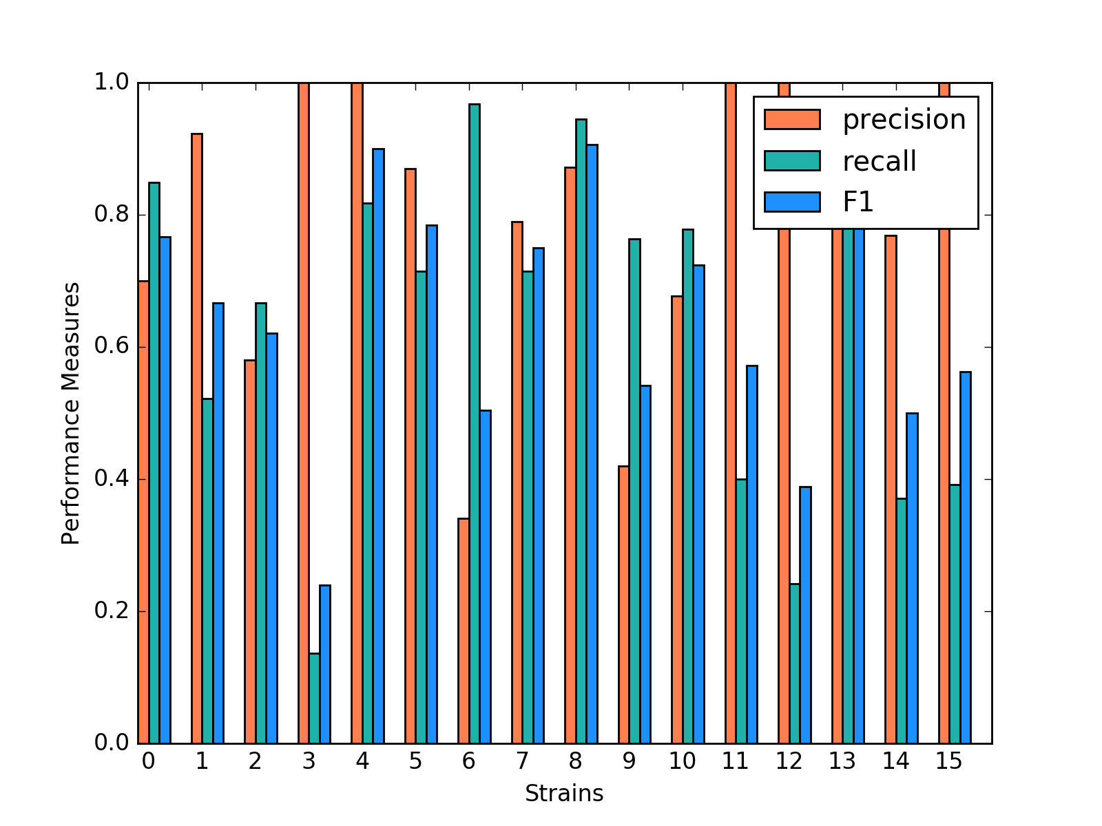
SVM model shows a very inconsistent performance on the prediction. For example, the precision for predicting strain 3,4,11,12,15 is 1 while the precision for predicting strain 6,9 is below 0.5. Although precision for predicting strain 3,11,12,15 is very high, the recall for predicting these strains are much lower, resulting in a low F-1 measurement. The high precision and low recall indicates that we can trust the classification judgements, however the low rate of recall indicates that SVM is very conservative. This might be good if we are worried about incorrectly classifying the strains.
(Source code, png, hires.png, pdf)
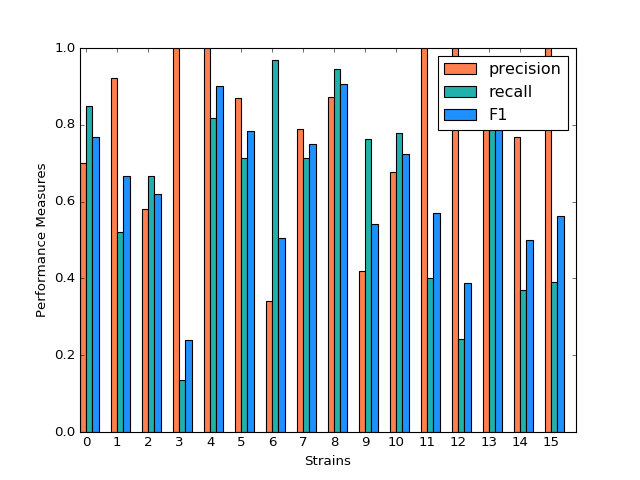
Classification Performance of SVM
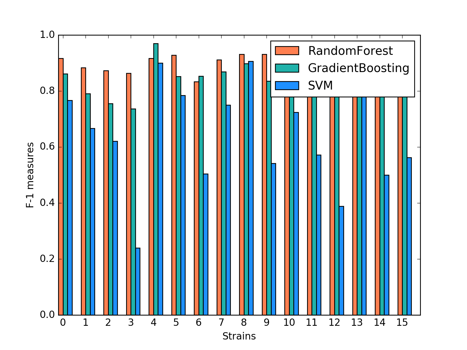
Comparison
By plotting side-by-side barplot of F-1 measurement among the three models, we can clearly see that Random Forest model provides the best result and SVM is the worst. Performance of Random Forest and Gradient Boosting are similar, but the SVM is obviously weak. So we recommend predicting strains by implementing the Random Forest model.
(Source code, png, hires.png, pdf)

Comparison of F1 measures of Different Classification Models
Clustering
K-means
The silhouette scores corresponding to the number of clusters ranging from 2 to 16 are: 0.835, 0.775, 0.423, 0.415, 0.432, 0.421, 0.404, 0.383, 0.421, 0.327, 0.388, 0.347, 0.388, 0.371,0.362. We plot 6 clusters here to show, and found that Czech and CAST mice behaved quite differently from each other.
Distribution of strains in clusters by K-means algorithm (Generated by plot_strain_cluster function; script can be found in report/plots directory.)
Hierarchical Clustering
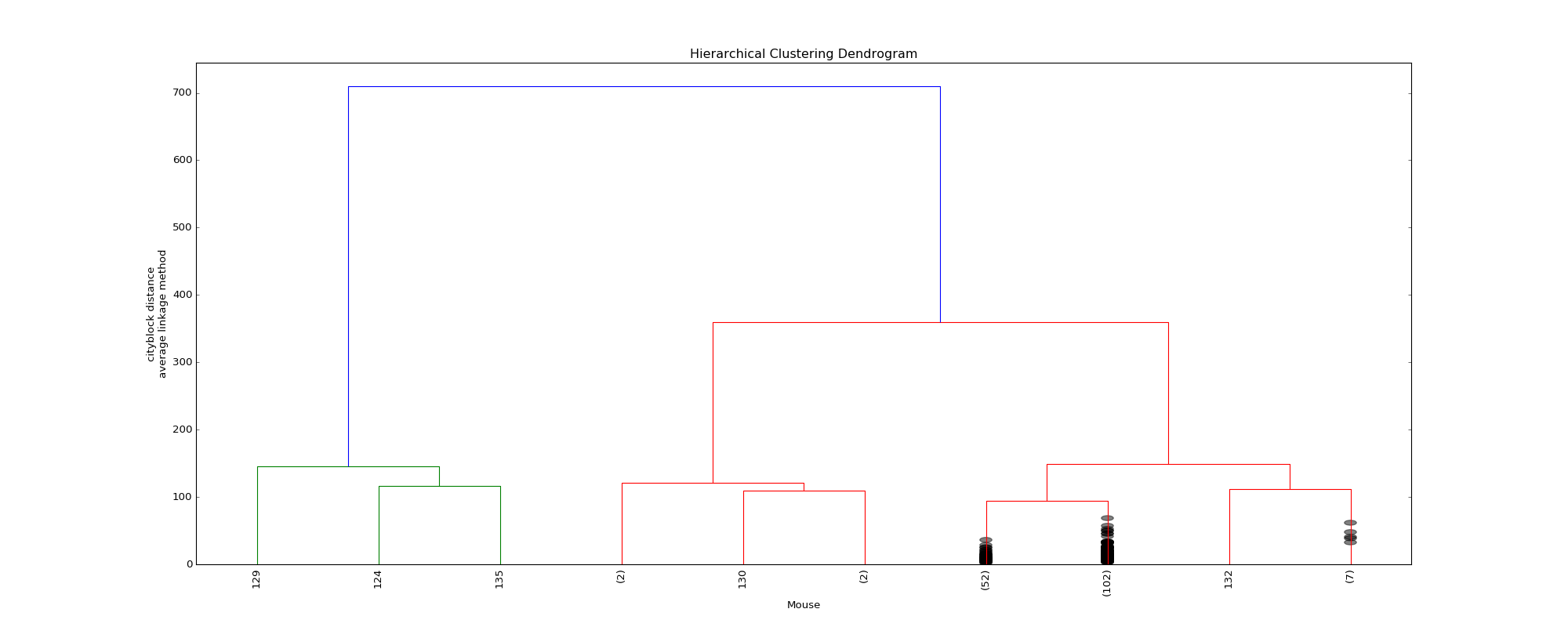
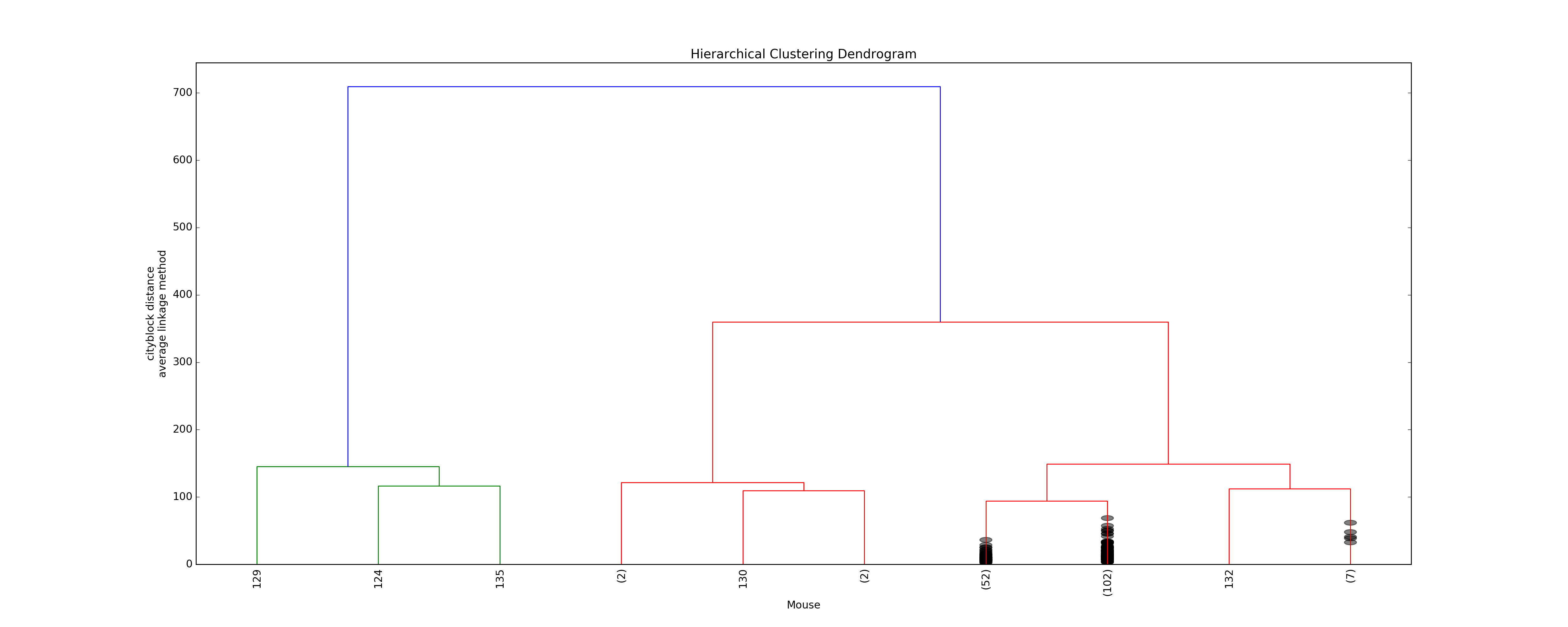
The optimal distance measure is l1-norm and the optimal linkage method is average linkage method. The silhouette scores corresponding to the number of clusters ranging from 2 to 16 are: 0.8525, 0.7548, 0.7503, 0.6695, 0.6796, 0.4536, 0.4557, 0.4574, 0.3997, 0.4057, 0.3893, 0.3959, 0.4075, 0.4088, 0.4179. It seems 6 clusters is a good choice from the silhouette scores.
However, the clustering dendrogram tells a different story. Below shows the last 10 merges of the hierarchical clustering algorithm. The black dots indicate the earlier merges. The leaf texts are either the mouse id (ranges from 0 to 169) or the number of mice in that leaf. Clearly, we see that almost all the mice are clustered in 2 clusters, very far from the rest individuals. Thus, the hierarchical clustering fails to correctly cluster the mice in the case.
(Source code, png, hires.png, pdf)

Dendrogram of the hierarchical clustering
The failure of the the algorithm might be due to the different importance levels of the features in determining which cluster a mouse belongs to. One improvement could be that using only the important features determined in the classification algorithms to cluster the mice, but given the unsupervised learning nature of the algorithm, not using the results from the classification is fair for clustering tasks.
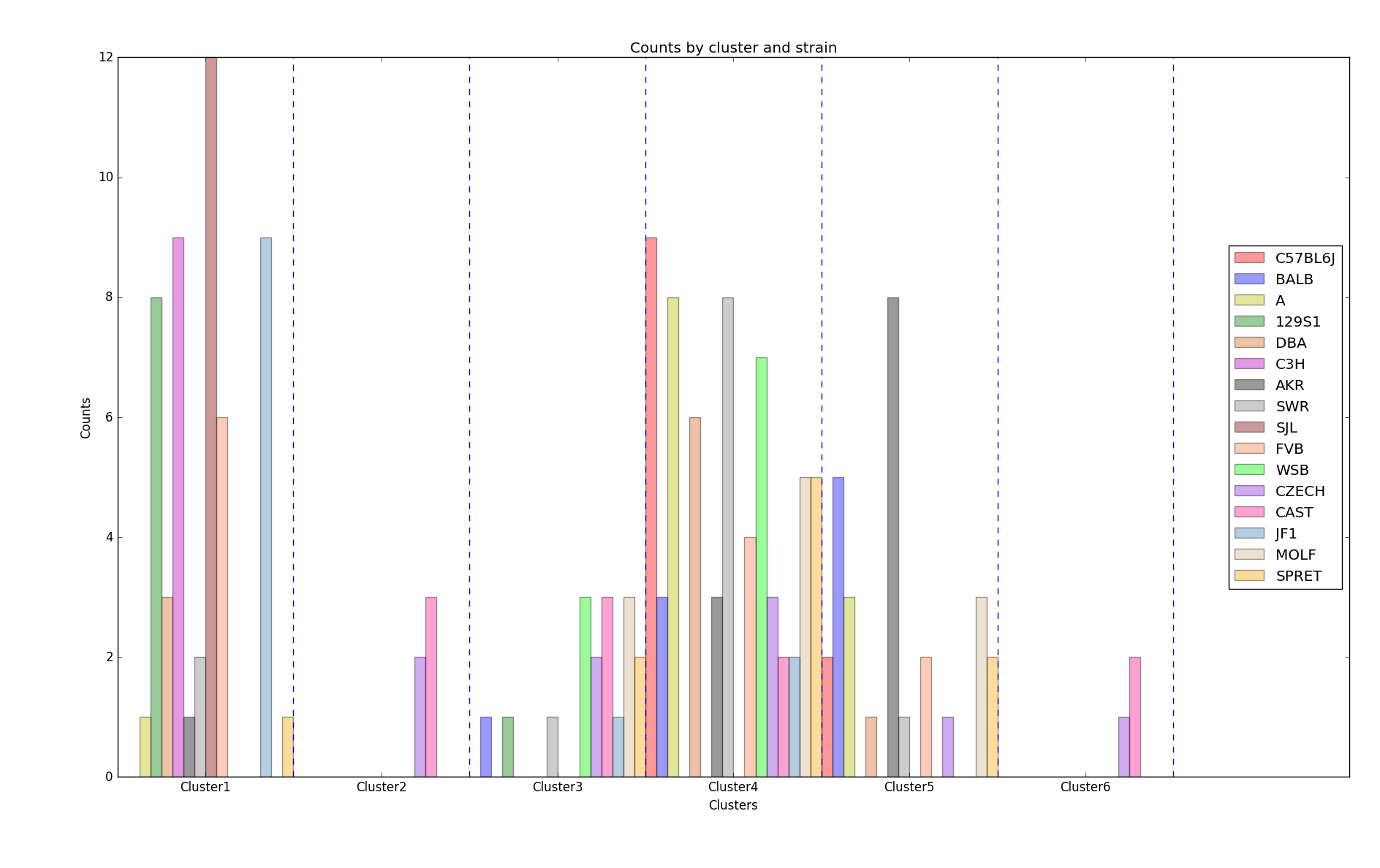
The distribution of strains in each cluster in the case of using 6 clusters are shown below. Obviously, the mice almost fall into the same cluster.
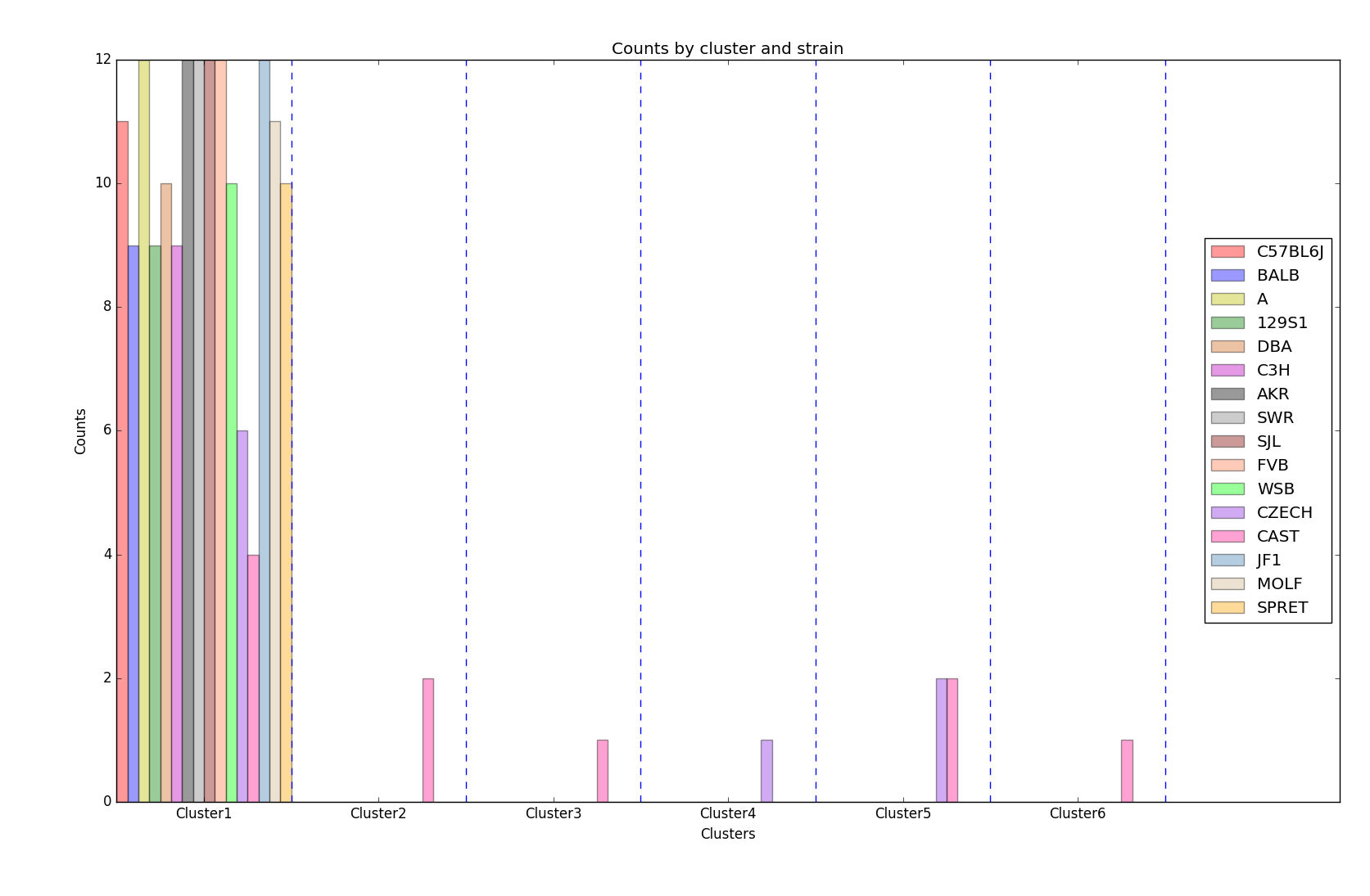
Distribution of strains in clusters by agglomerative hierarchical clustering (Generated by plot_strain_cluster function; script can be found in report/plots directory.)
Future Work
The future research should focus more on feature engineering, including the questions of whether more features could be added to the model. Moreover, even though we have extracted the important features from the random forest to evaluate the performance of the smaller model, it seemed that the economized model did not perform as expected. In the future, other techniques like PCA might be performed to reduce the complexity of the model in order to train classification models faster.
To understand more about the nature of the strain difference, it would be better to have a sense of relationships between different strains of mice. For instance, we have explored that these 16 strains of mice belong to 7 different groups, which implied that some strains were genetically similar. Considering the time limit, we have put it to the future work.