Power Laws and Universality

Statement of Problem

Construct Statistical Model for Locomotion Distribution

To take a closer look at the tail property of locomotion, we analyze the moving distance distribution for each string. Fitting those distributions using some prior knowledge and obtain estimator for each mouse. With expectation, it is possible to cluster mice by the their unique distribution estimator, and further figure figure out with strain they belong to.

Main Questions to Answer

• What is the distribution model we could use to fit?
• How can we estimate parameters for our distribution?
• How can we do clustering strains based on model parameters?

Statement of Statistical Problem

Distribution Selection

The major statistical question is how to choose fitted distribution family. Based on conventions and data we have, we propose two distributions: law decay distribution and exponenital distribution:

In statistics, power law, also known as a pareto, is a functional relationship between two quantities, where a relative change in one quantity results in a proportional relative change in the other quantity, independent of the initial size of those quantities: one quantity varies as a power of another. \(F(x)=kx^{-a}\).

There is a problem with power law or pareto distribution when took a close look at the distance distribution. This power law decay only works for monotone decreasing distribution. While it is not for our case. Therefore, two methods are designed to handle this.

First of all, we proposed to only estimate the powerlaw on the tail of distribution. Namely, truncate the small unstable distances on the left tail of distribution. Secondly, the power function may not be realistic by nature as the observed distribution is not monotone decreasing. In this case, the distribution is left skewed with one peak (see exploratory analysis). Thus we can make more general assumption, such as exponential distribution.

Fitness Comparsion

Previously we proposed two different parametric families and each of them make sense but we need to have more quantitative evidence to see the fittness or, hopefully, compare their goodness of fit.

The check of fitness is in needed after obtaining the parameter. Kolmogorov-Smirnov test enable us to test the fitness of power law and exponential distribution. For them, we choose the null to be selected distribution, and if we reject K-S test, we will conclude the the sample distribution is not familiar with theoretical distribution; thus, we have enough evidence against our null.

After that, to further compare these two distribution’s capability of capturing the pattern of distances, we conducted a generalized likelihood ratio test (GLRT), with both two to be null hypothesis consecutively. Moreover, it may be hard to know the exact distribution of our test statistics and thus extremely hard to calculate the critical value or p-values. Therefore, we may need simulation methods to estimate critial value of p-value, and the major question is how can we generate random number from our fitted model.

Exploratory Analysis

The difference between “home base” and “non home base”: “home base”, which means a favored location at which long periods of inactivity (ISs) occur, is a post defined characteristic of the mouse and it is classified by its behavior. For instance, if one mice spend about 80% of the time outside of the nest, then we may conclude it is not home base and we will cluster it as non-home based mouse. This classification is not done by one specific mouse, but a strain of mouse. By the Exploratory Analysis, we will find significant difference between two classes and hopefully we can make connection about the speed of mice and its home based or non home based property.

The definition of inter-event distance: literally, inter-event distance is the distance within one single event. Investigating the data of the distance between each two consecutive points recorded by the detector of one mouse day, we found the shape of the histogram is similar to the plot on the slide, except the value of frequency is bigger. This inconsistency gives us the motivation to calculate the inter event distance instead of the distance between each two points. For this purpose, we need a vector of the index of events for each mouse day. In particular, the mapping vector is connected by time since xy coordinates are recorded according to time and the event is defined based on time.

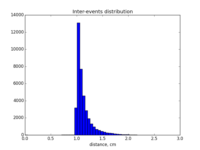
Preferred choice of distribution: the power law is a monotone decreasing, however our plot indicates a peak. Therefore, we can either choose differernt parametric distribution family, such as gamma distribution, or choose a threshold to make our distribution monotonic decreasing. Based on what Chris said about the sensor, as it will only detect when a mice moves more than 1cm within in 20ms. It does not make sense to have observations less than 1cm and outliers needs to be cleaned up. After we put a threshold with 1cm, we find the distribution is monotonic decreasing and we can fit power law distribution, as well as exponential distribution.

Distribution

• Preferred choice of distribution: the power law is a monotone decreasing, however our plot indicates a peak, in which gamma distribution may fit better.
• Another idea would be to record the position of the mouse at regular time intervals and compute the distances between them. This will give us an idea of the speed distribution of the mouse.

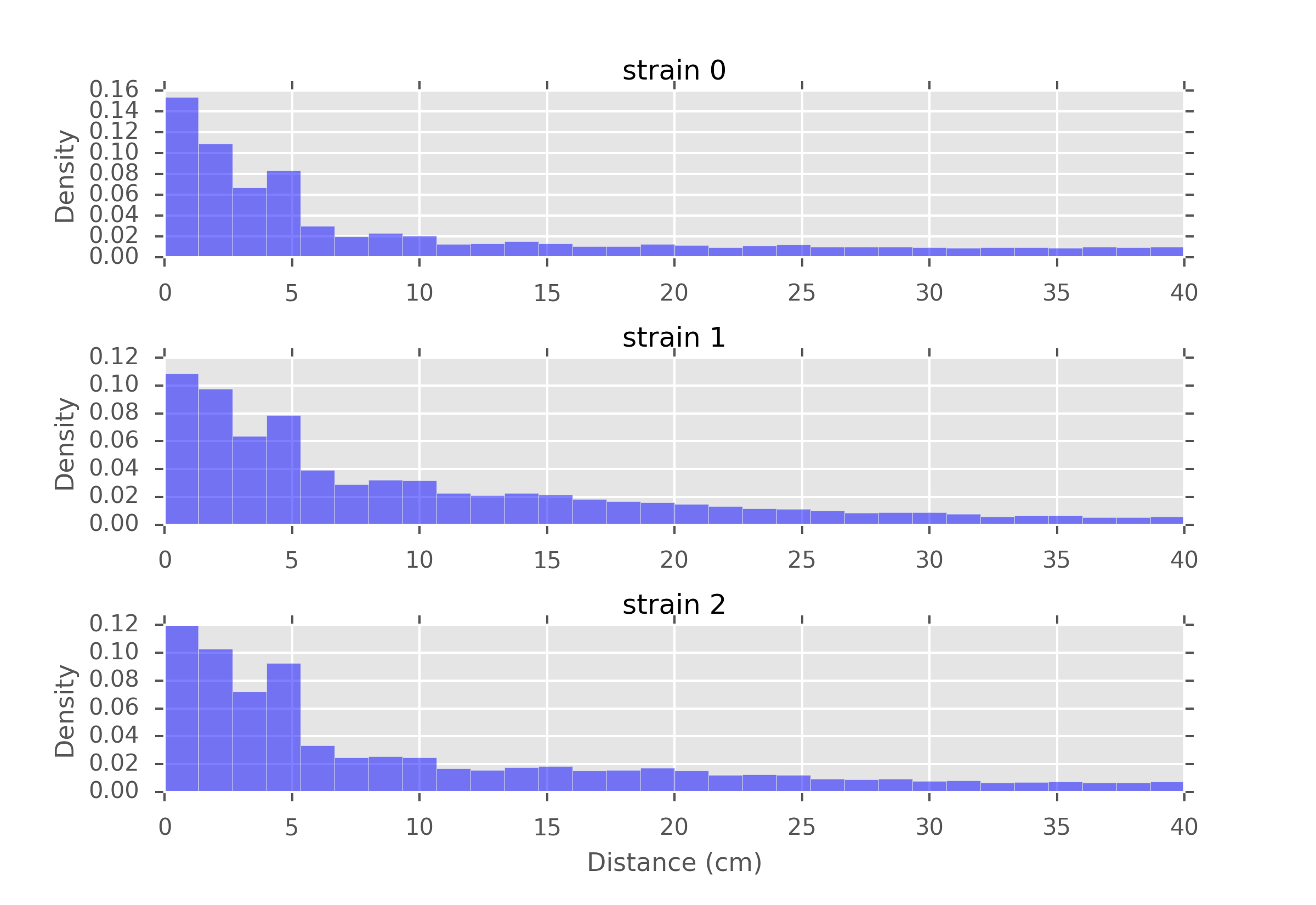
Distances recorded every second, for different strains of mice

Data Requirements

• Label of “home base” or “non home base”: generated in the process of data pre-processing by the definition. The build-in function enable us load data directly.
• Event index corresponding to the time: a vector mapped the time indicating the events.
• Distance: calculated by the square root of the sum of the difference x,y coordinates
• Speed: calculated by the distance divided by the duration of this distance.

Methodology

Given the estimated parameter for each distribution, we can learn more about its distribution and the information lies mainly in the decay rate of the tail.

Here are our algorithms:

• Draw the histogram for our data. For each mouse day, observe the distribution and explore whether our distribution assumption makes sense.

• Estimate parameters based on MLE of truncated powerlaw, aka Pareto distribution and truncated exponential.

• Add the density function to our histogram, see the fitness of our distribution.

• Conduct statistical test to quantitatively analysis the fitness. For testing the hypothetical distributions of a given array, there are several existing commonly used methods:

  • Kolmogorov–Smirnov test
  • Cramér–von Mises criterion
  • Anderson–Darling test
  • Shapiro–Wilk test
  • Chi-squared test
  • Akaike information criterion
  • Hosmer–Lemeshow test

  However, each approach has their pros and cons. We adopt KS test since the Kolmogorov–Smirnov statistic quantifies a distance between the empirical distribution function of the sample and the cumulative distribution function of the reference distribution. We recommend that all the methods are to be tried to get a comprehensive understanding of the inter-event step distributions.

• Conduct Generalized Likehood Ratio Test to compare the fitness of powerlaw and exponential. GLRT will calculate Likelihood Ratio which is the fraction of likelihood function with smallest KL divergence in two separate parametric space and then compare their peroformance.

Testing Framework Outline

The potential functions are recommended to implement:

• Retrieve data function (retrieve_data): Given the number of mouse and the date, create a data frame containing follow variables. 1) position: x,y coordinates 2) time: detecting time stamp for each pair of coordinates, time interval label for events, time interval label for active state and inactive state.

• Retrieve event function (retrieve_event): Given an event label (e.g. Food), subset respective part of data from the data frame we got in retrieve_data

• Compute the distance (compute_distance): Given event label, compute the distance between each time stamp. As we already know the x, y coordinates from the dataframe in retrieve_event, the simplest way to implement this function is that:

  \[distance = ((x_t2 - x_t1)^2+(y_t2 - y_t1)^2)^(1/2)\]

• Draw histogram (draw_histogram): Given a sub-array, using the plt built-in histogram function to draw the plot. Test distribution (fit_distr): Given the testing methods (e.g. “ks”), implement the corresponding fitting methods. The potential output could be p-value of the hypothesis test.

Based on the potential functions to be implemented, the following is the guide of testing:

• test_retrieve_data: attain a small subset of data from x,y coordinate and t, and feed in the function. Compare the results with the counted number.
• test_retrieve_event: Use the small data frame we get in test_retrieve_data, given different events/state. Compare the results with our counted number.
• test_compute_distance: Given x = 3, y =4, the output should be 5.
• test_fit_distr: randomly draw samples from widely used distributions (e.g. uniform). Test it with right(e.g. uniform) and wrong(e.g. gamma) distributions. Compare the p-values with given threshold (e.g. alpha = 95%)

Result

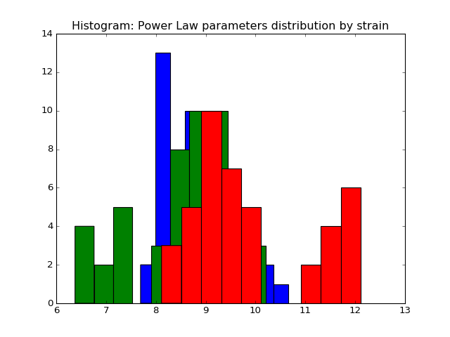
We fit the power law and exponential distribution for each mouse day. For each, we got an estimator of alpha for power law and an estimator of lambda for exponential. We store our result in a dataframe called estimation which has five columns: strain, mouse, day alpha and lambda. Draw histogram of the estimator where red, blue and green stands for different strains.

• The histogram of estimators from powerlaw:

(Source code, png, hires.png, pdf)

Histogram of the parameters of powerlaw.

• The histogram of estimators from exponential:

(Source code, png, hires.png, pdf)

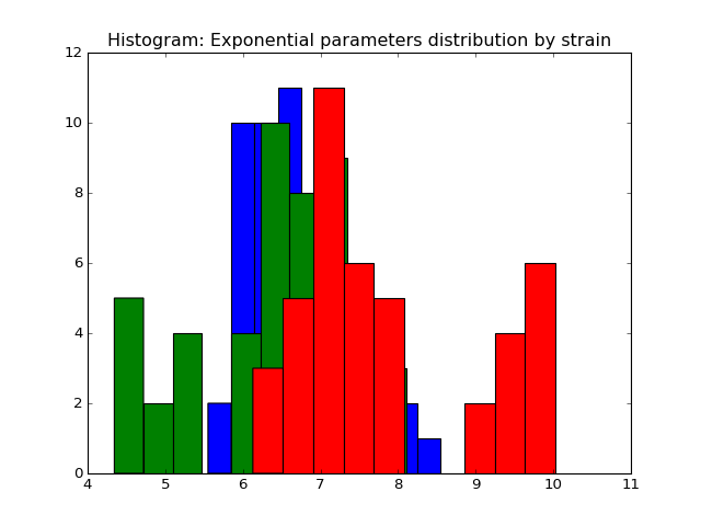
Histogram of the parameters of exponential.

We want to check the fitted curve with the original histogram of distance so we write of function to draw the power law and exponential curve with corresponding estimator with the original histogram of distance with the input of strain, mouse and day. In particular, some normalization may be needed when doing the camparison and drawing the plot, for example, we intutively times (alpha-1) for the histogram. Here is an example of strain 0, mouse 2, day 5. From the plot we can see the fitting is pretty well.

• The histogram of data and fitted curve for strain 0, mouse 2, day 5:

(Source code, png, hires.png, pdf)

Histogram and fitted curve for strain 0, mouse 2, day 5.

After visualize the fitting, we want to evaluate our fitting in statistical ways. There are several tests to quantify the performance and we adopt the KS test to evaluate the goodness of fit and GLRT test to compare fitness.

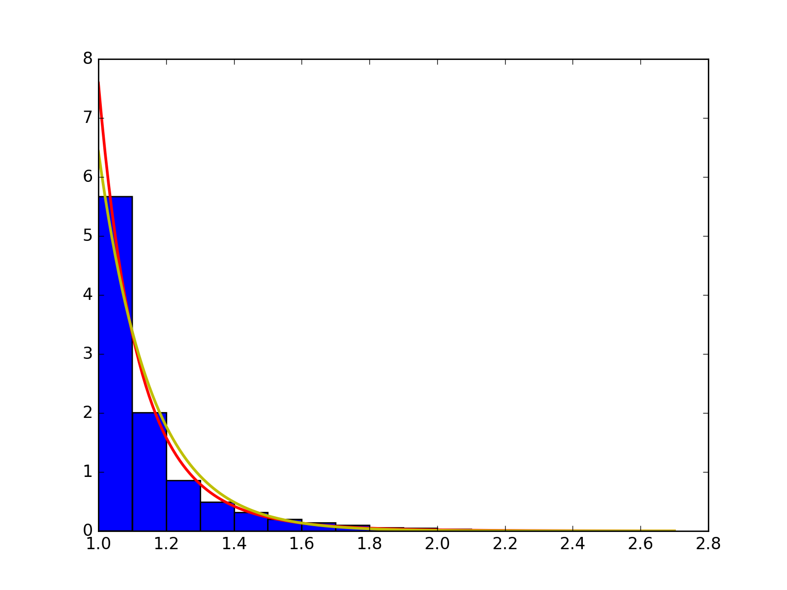
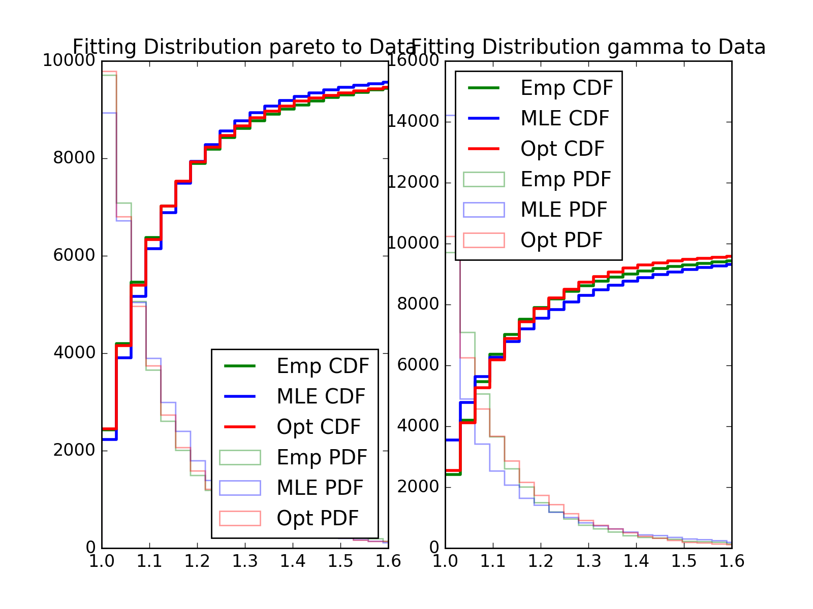
• Fitting power law distribution and gamma distribution for strain 0, mouse 0, and day 0; fitting by Maximum Likelihood, and by minimizing Kolmogorov CDF distances:

(Source code, png, hires.png, pdf)

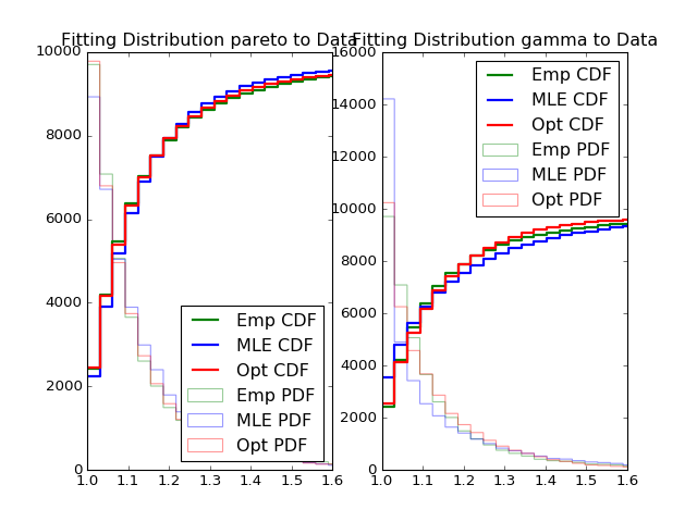
Histogram of distances travelled in 20ms by strain 0, mouse 0, day 0.

• Comparsion Between truncated Exponential and Powerlaw (Pareto) distribution.

One major question we want to answer: which distribution fits better, truncated exponential or truncated power law, aka pareto, distribution. To measure the distribution of the speed, the major difference is the tail distribution. You can also see it from the fitted plot. Both exponential distribution and pareto distribution fits quite well and they are actually very similar with each other, and the difference is barely noticeable. Therefore, it is hard to simply tell which distribution fits better. However, although the distribution is quite similar at the beginning, it diverse in the tail distribution. For exponential distribution, the tail decays with the rate e^{-x}, which is much faster than that of pareto distribution x^{-a}. Therefore, the goodness of fit is mainly determined by the tail distribution. We tried Kolmogorov test to determine whether our sample fits the theoretical distribution, but it does not compare two distributions.

To make comparison between two distributions, we used Generalized Likelihood Ratio Test to do hypothesis testing. As we cannot actually treat different distribution equally, with that being said, to do hypothesis testing, we must have null hypothesis and alternative hypothesis, where we tend to protect it and only reject when the we have strong evidence against it. Thus, we will conduct two hypothesis testings, with null being either exponential or power law distribution. We will expect there to be three possible outcomes.

• Exponential null rejected but power law null not rejected. In this case, we conclude power law is better than exponential.
• Power law null rejected but exponential null not rejected. In this case, we conclude exponential is better than power law.
• Both two tests not rejected. In this case, we conclude both two fits similarly and there is no one significantly better than another.

Although theoretically we should consider the case when both two tests are rejected, it is highly unlikely this thing happens. Because rejecting both two means we have enough evidence to say exponential is better and power law is also better, while not rejecting two might happen, as we tends to protect the null and if they react similarly, we don’t have enough evidence to reject any of them.

Here is the algorithm to conduct the test. The GLRT test statistics is the ratio of likelihood, with numerator being likelihood under null set while that under alternative in numerator. It is intuitively right that we shall reject the null if our test statistics is too small. To make the significance level being 0.05, it is essential to find the critical value. However, it is hard for us to derive the distribution of test statistics and thus we use simulation to estimate it. Thus, we draw random number from null distribution and then calculate the test statistics. Also, p-value is a better statistics and it will not only tell us whether we should reject the null, but also tell us what is the confidence that we reject the null.

From the outcome of our function, we actually find the p-value from exponential null is very close to 1, while that from power law null is very Small, next to 0.0005. This is a strong evidence that we should not think power law is a better fit than exponential. Thus, we conclude that we should use exponential to fit and do further research.

Relative distribution with kernel smooting

In the previous section, the result of K-S test suggests that the actual distribution of distance doesn’t follow the power law family but may follow in the exponential family. In this section, we characterize discrepency of the actual distribution to these two by looking at their relative distribution.

In the relative distribution framework, we call the actual distribution \(G\) comparison distribution and call the proposed distribution \(F_0\), e.g. power law with parameter \(\alpha\), the reference distribution. The idea of the relative distribution is to characterize the change in distributions by using \(F_0\) to transform X into \([0,1]\), and then look at how the density departs from uniformity.

The relative data, or grades, are \(r_i =F_0(x_i)\), which lies in \([0,1]\). Its probability density function is $f_r(x) = frac{g(F_0^{-1}(x))}{f_0(F_0^{-1}(x))}$. \(r\) has uniform density in the special case when \(G = F\).

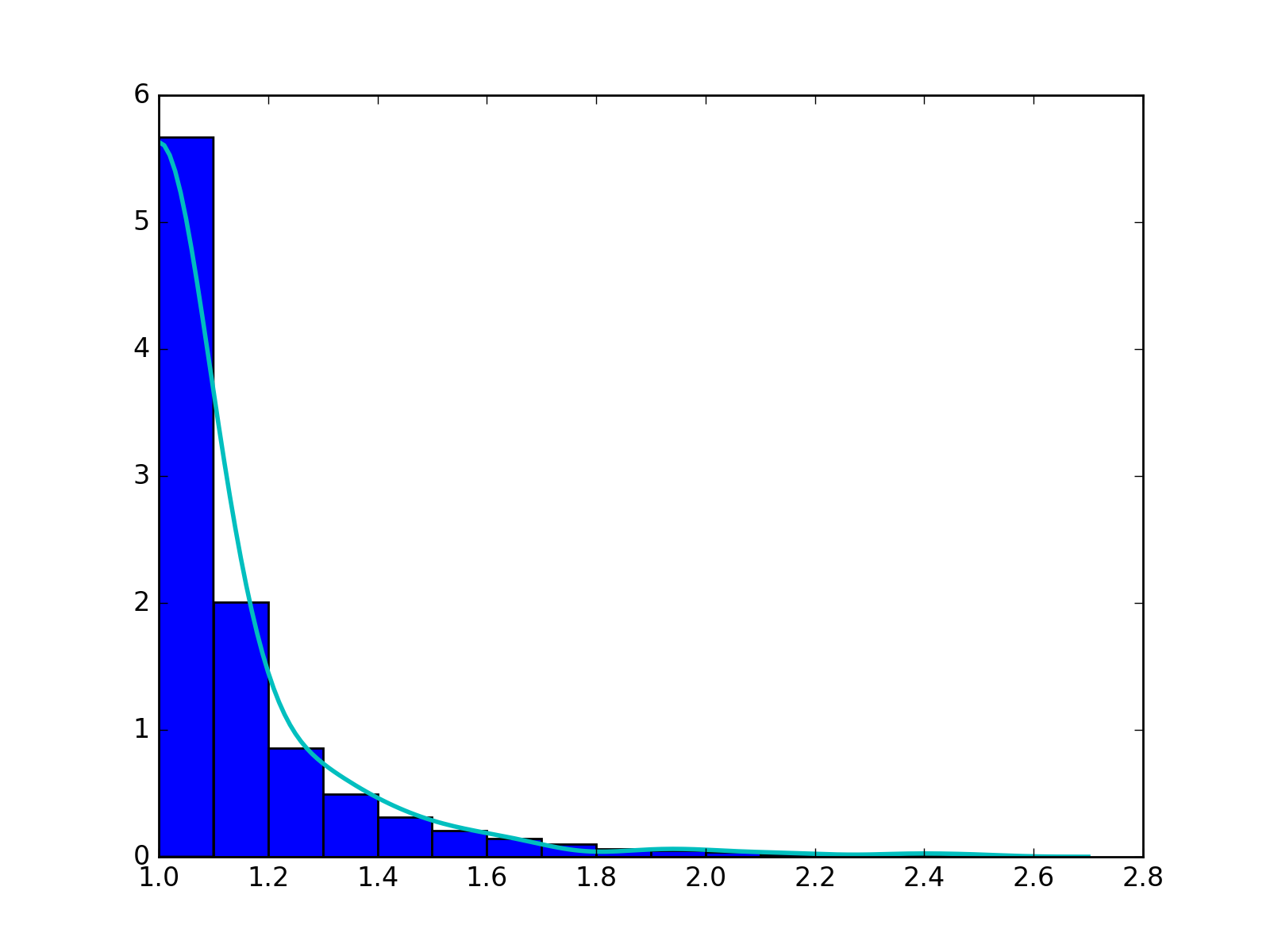
As shown in the previous formula, we need to get the density \(g\) of the observed data to calculate the relative distribution. However, the naive nonparametric density estimation with gaussian kernel doesn’t work well when the random variable is nonnegative. We propose a strategy using symmetric correction to work it around.

In the first step, we create the symmetric-corrected data \(X'\) by concatenating the original data \(X\) and its reflection around its left boundary point 1, \(2-X\). In the second step, we get \(f_1\), the density estimate using gaussian kernel with bandwidth maximizing 5-fold cross-validated score. In the third step, we delete \(2-X\) and set the density estimate of \(X\) to be \(f=2f_1\). An example is shown in the plot.

(Source code, png, hires.png, pdf)

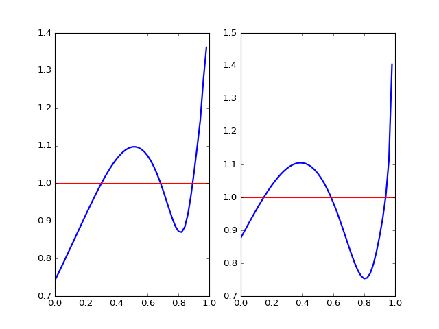
We construct the relative distribution to the best-fitted power law distribution and exponential distribution using this density. The result is shown in the plotted density curve.

(Source code, png, hires.png, pdf)

Relative distributions, power law on the left, exponential on the right

Now, the fine relative density structure is very clear. We see our actual distribution has a smaller density at the beginning and a thicker tail compared to both power law distribution and exponential distribution. Exponential has a better fit at the beginning and a worse fit for the tail, which gives rise to smaller discrepency in CDF and smaller K-S statistic. However, neither family seems to be good enough in terms of density characterization of distribution.

Mann-Whitney U test on distances

Given the distribution of distances, we perform a hypothesis test on the distributions of these distances. The goal is to identify some similarity on mice in the same strain when only looking at the distances covered every second.

To do so we chose a non parametric test since we only have access to sample distributions. The Kolmogorov Smirnov test is a very popular test used in this case but I chose to explore the Mann-Whitney U test instead for the following reasons:

• The KS test is sensitive to any differences in the two distributions. Substantial differences in shape, spread or median will result in a small P value. (see here for more details). Here we can feel that the distances have high variance. Therefore, the KS test would be too strict for our study.
• In contrast, the MW test is mostly sensitive to changes in the median, which is less sensitive of noise in the case of mice.

The MannWhitney U test is a test for assessing whether two independent samples come from the same distribution. The null hypothesis for this test is that the two groups have the same distribution, while the alternative hypothesis is that one group has larger (or smaller) values than the other.

• \(H_0$: $P(X>Y)=P(Y>X)\)
• \(H_1$: $P(X>Y)\neq P(Y>X)\)

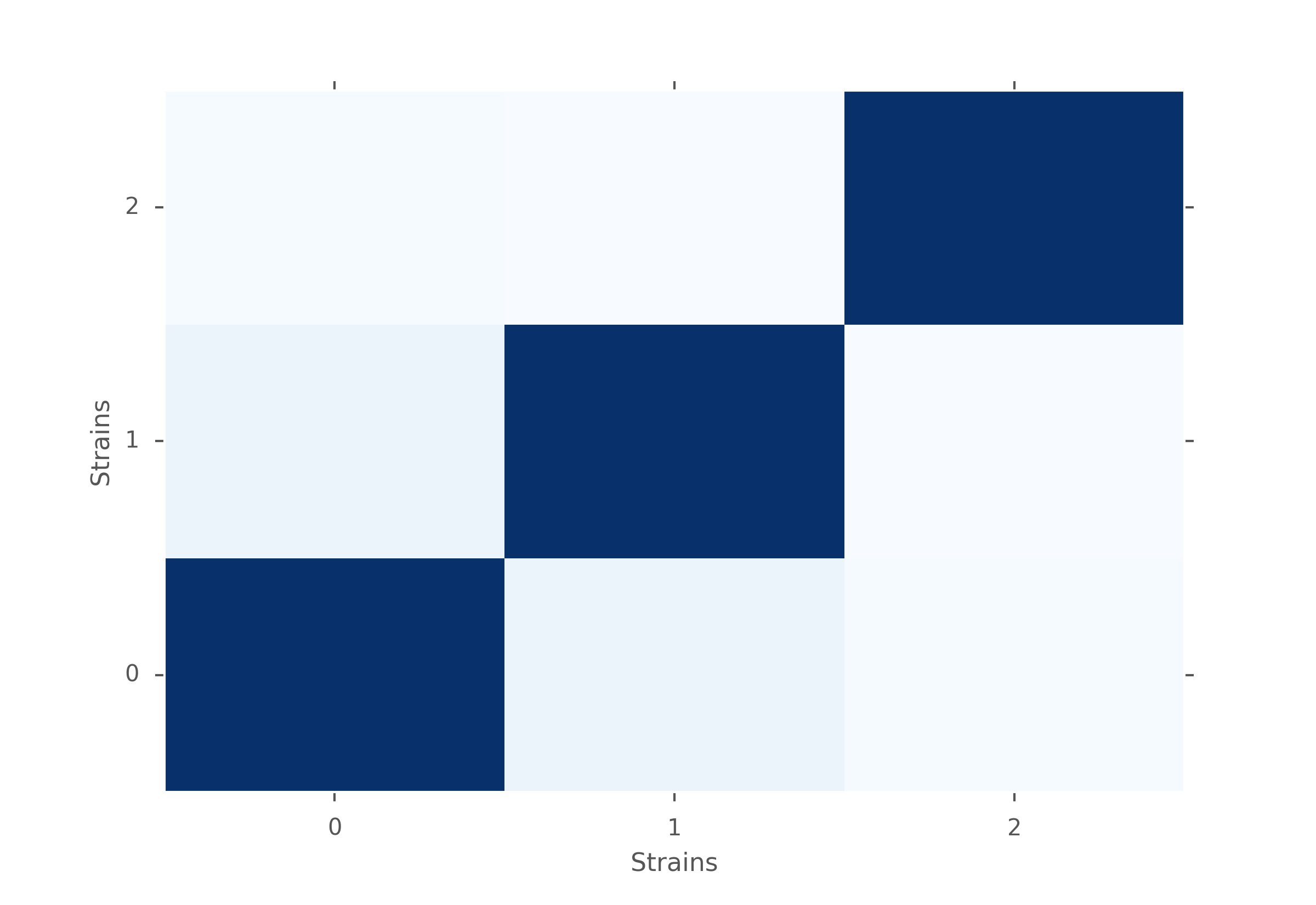
MW U test p-values for different strains of mice. Dark blue is close to 1 and very light blue is close to zero.

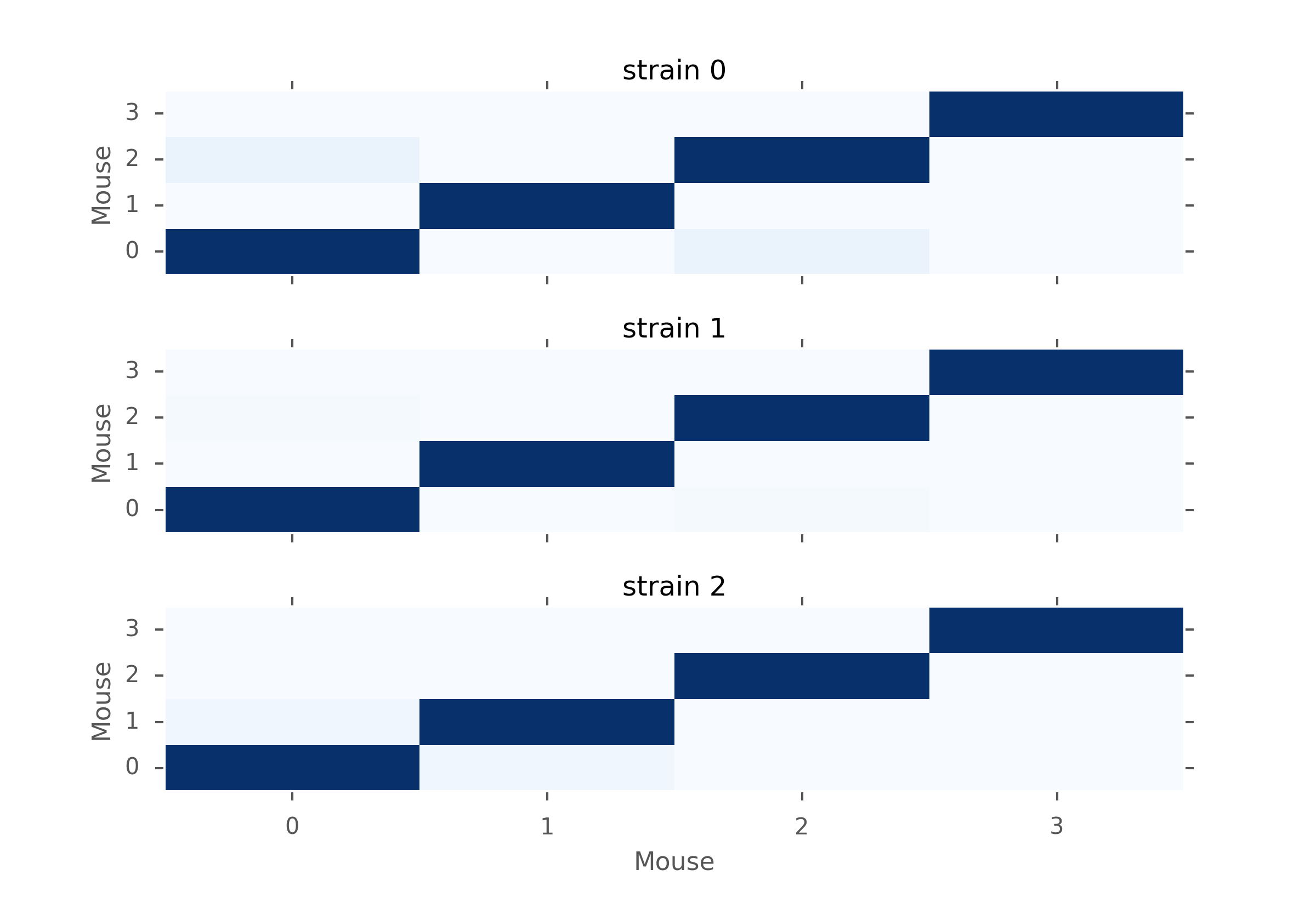
MW U test p-values for mice within the same strains. Dark blue is close to 1 and very light blue is close to zero.

From the figures above, we notice that in terms of p-values, strain 1 is closer to strain 0 than strain 2. But we also notice that the p-values are still very low, which means that there is evidence for rejecting \(H_0\). Moreover, when looking closer within each strain of mice, we can see that mice have different distributions too. Therefore, based on the inter-distances, we cannot conclude that mice behave similarly depending on their strains.

Future Work

Here are some further research we could do. However, because of Incomplete sample we have, we cannot do it for now, but it is easy to fix the function

• K means clustering:

One major goal of this project is to measure similarity between different strain and hopefully make clusters based on our data. But one difficulty is that we cannot plug in the information we have to a known machine learning clustering algorithm. However, as truncated exponential to be a good fit. We can use the parameters to measure the similarity and transform our sample data to one scalar. One classic unsupervised learning algorithm is K-means and we can definitely use it to make clusters. However, one drawback is the distance between our parameters is not uniform but as long as there exists significant difference, it will not harm that much.

Reference reading

• https://en.wikipedia.org/wiki/Power_law
• http://arxiv.org/pdf/0706.1062v2.pdf