Ultradian and Circadian Analysis
Statement of Problem
Ultradian and circadian rhythm are widely observed in mammalian behavioral patterns. The ultradian analysis aims to find the time-specific patterns in behavioral records, without specifying the length of the cycle in advance (but need to be within 1 hour to 1 day). The typical ultradian period includes 8 and 12 hours. The circadian rhythm refers to a roughly 24-hour cycle. For example, we expect the rats to be inactive in the nighttime and ingestions and movements mostly happened in the daytime.
The variables of interests are the summary statistics of mouse activity including food (F) and water (W) ingestion, distance traveled (D), Active State probability (AS), movement inside the home base (M_IS) and movement outside the home base (M_AS). We may also consider spatial variables, for example, we can spatially discretize the data to cells containing the primary functions, like a food cell or a water cell, and examine the ultradian cycle of the spatial probability densities of the occupancy time in each cell.
In this report, we assume strain to be the primary influence on the variation of ultradian rhythms across individual mice and examine the difference in rhythms across strains. Currently, we lack basic information such as weight, age, and gender. With more data available in the future, we may look into the cycle for each mouse and detect the most important factors influencing the ultradian rhythms.
The ultradian and circadian analysis is closely related to other subprojects. Ultradian rhythms could be treated as one feature for clustering the 16 strains. We may also subset the data using the results of the cluster and analyze the rhythm similarities and differences across clusters.
Statement of Statistical Problem
Our statistical problems are three parts: data preparation, choice of the frequency or period, and modeling of rhythm patterns.
Data preparation:
Mouse behaviors are recorded based on time intervals or time points, like the beginning and ending time stamp of one food ingestion or the coordinates of mouse position at a particular time point. We aggregate the data based on given time bins and thus convert the raw data to time series. Then how to determine the optimal bin intervals for constructing the time series? Bin interval examples include 5 min, 30 min, 1 hour, etc.
Choice of the frequency or period:
For ultradian rhythms, the significant period length may vary according to the variables of interests. The Lomb-Scargle (LS) periodogram spectral analysis technique, a widely used tool in period detection and frequency analysis, is applied.
Modeling of rhythm patterns:
We are not only interested in the period length of circadian and ultradian rhythms, but also the variation of features over time within the discovered circles. To model the time trajectory of features, we propose to use seasonal decomposition and mixed effects model.
Data
In order to retrieve the data needed for analyzing mouse ultradian behaviors, we get input from users, including features (water, food, active state, etc.), strain number, mouse number and time bin width. Also, we have another function called “aggregate movements” to track mice’s movements intensity based on time bins. They enable us to specify which mouse and which kind of features to study. After getting bin width from users, we allocate the time used by each feature into selected time intervals. For example, if “30 minutes” is selected to be bin width and “food” is selected to be the feature, then the eating time intervals are separated are relocated into 30-minute long bins. For one mouse day, using 30-minute time bin gives 48 records as a result in total.
For eating and drinking behavior, instead of using time consumption as intensity, we choose to use food or water consumption amount by acquiring food/water consuming data, and assuming the food/water expended during feeding is proportional to the time used. For calculating the movements data, we figured out the position change by generating Euclidean distances first and then distributing them into different time bins.
The output is a pandas time series, with time index representing time intervals and values including feature data (such as food/water consumption, active state time as well as movement distance).
- Input:
records for each strain (total of 16), each feature of interest (food, water, distance, active_state probability, ...), in a duration of 12 days (excluding 4 acclimation days).
- Processed:
using one-minute time bins of movement records to binary score the activity into 0 (IS: inactive state) and 1 (AS: active state); using thirty-minute bins of food records to calculate the amount of chows consumed by mice; using LS periodogram technique to select the appropriate time bins for above.
- Output:
different patterned visualization for each feature, with the appropriate time bins that present the most significant ultradian pattern.
Methodology
Seasonal decomposition
Seasonal decomposition is a very common method used in time series analysis. One of the main objectives for a decomposition is to estimate seasonal effects that can be used to create and present seasonally adjusted values.
Two basic structures are commonly used:
1. Additive:  x_t = Trend + Seasonal + Random

2. Multiplicative:  x_t= Trend * Seasonal * Random
The “Random” term is often called “Irregular” in software for decompositions.
Basic steps:
1. Estimate the trend

2. "De-trend" the data

3. Estimate seasonal factors by using the "de-trended" series

4. Determine the "random" term
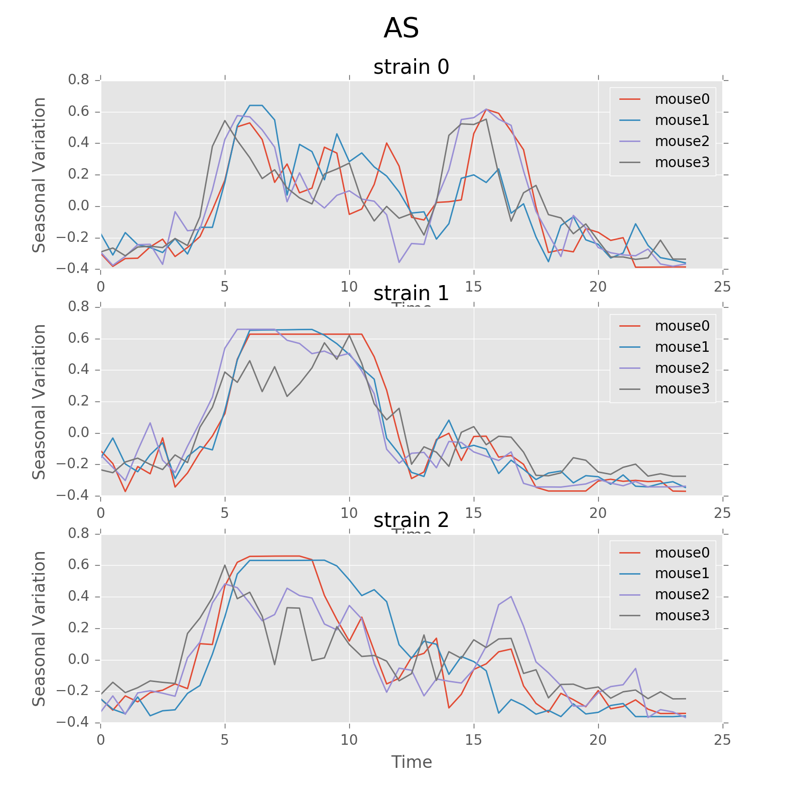
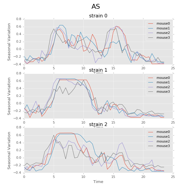
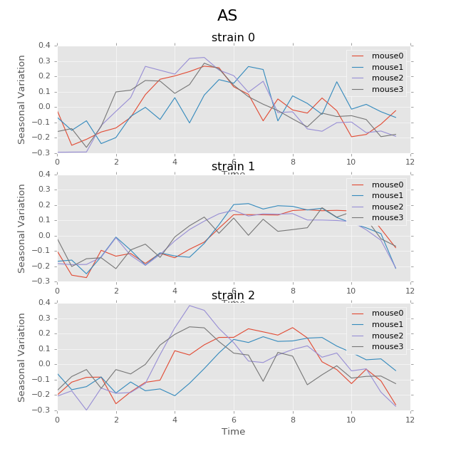
The following plot shows the seasonal variation of AS using circadian period. The difference between strains in rhythm patterns is evident.
Seasonal variation of AS probability (circadian, 24 hours). There appear to be significant patterns within each group. Strain0 tend to have two active stages every day, while strain1 will only have one active stage that lasts about 5 hours. The pattern in strain3 is not as strong as other strains, for that different mice seem to have larger variations. Nevertheless, the behavior with periods of 24 hours can be more regularly distributed than other periods showed below.
(Source code, png, hires.png, pdf)
Lomb-Scargle Period Test
Similar to Fourier analysis, the Lomb-Scargle periodogram is a common tool in the frequency analysis of unequally spaced data equivalent to least-squares fitting of sine waves. Basically, we want to fit sine waves of the form:
While standard fitting procedures require the solution of a set of linear equations for each sampled frequency, the Lomb-Scargle method provides an analytic solution and is therefore both convenient to use and efficient. In this case, we want to test whether each mouse/strain has a significant cycle less than 24 hours.
For the mouse behavior data, we use Lomb-Scargle method on different strain and mouse’s data to find the best possible periods with highest p-values. The function can be used on specific strains and specific mice, as well as just certain strains without specifying mouse number. We use the \(O(N\log N)\) fast implementation of Lomb-Scargle from the gatspy package, but the LS power around \(0\) period is a little bit noisy. The other algorithm can give smooth results around \(0\) point but suffer \(O(N^2)\) time complexity. Also, we need to add small uniformly distributed noise on the regularly sampled time sequence to avoid singular matrix problems.
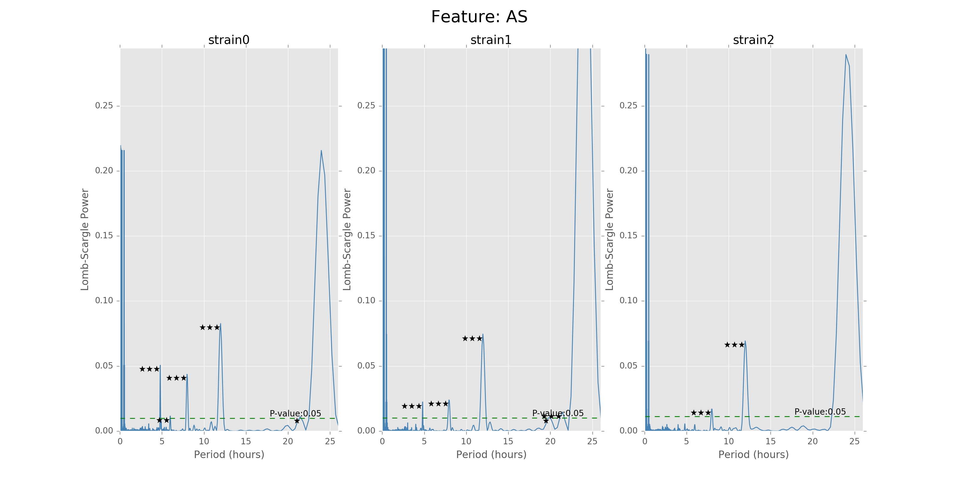
The function can give the LS power as well as the P values for the corresponding periods, with respect to the time bins chosen to combine the data. There will also be stars and horizontal lines indicating the p-values of significance. Three stars will be p-values in [0,0.001], two stars will be p-values in [0.001,0.01], one star will be p-values in [0.01,0.05]. The horizontal line is the LS power that has p-value of 0.05.
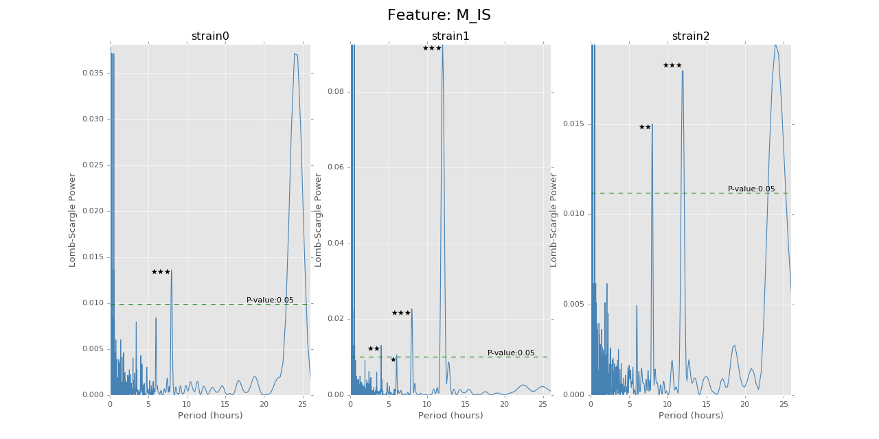
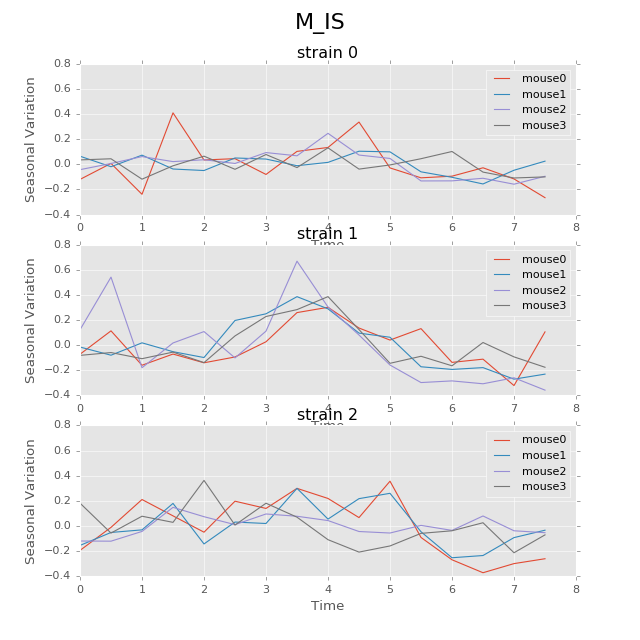
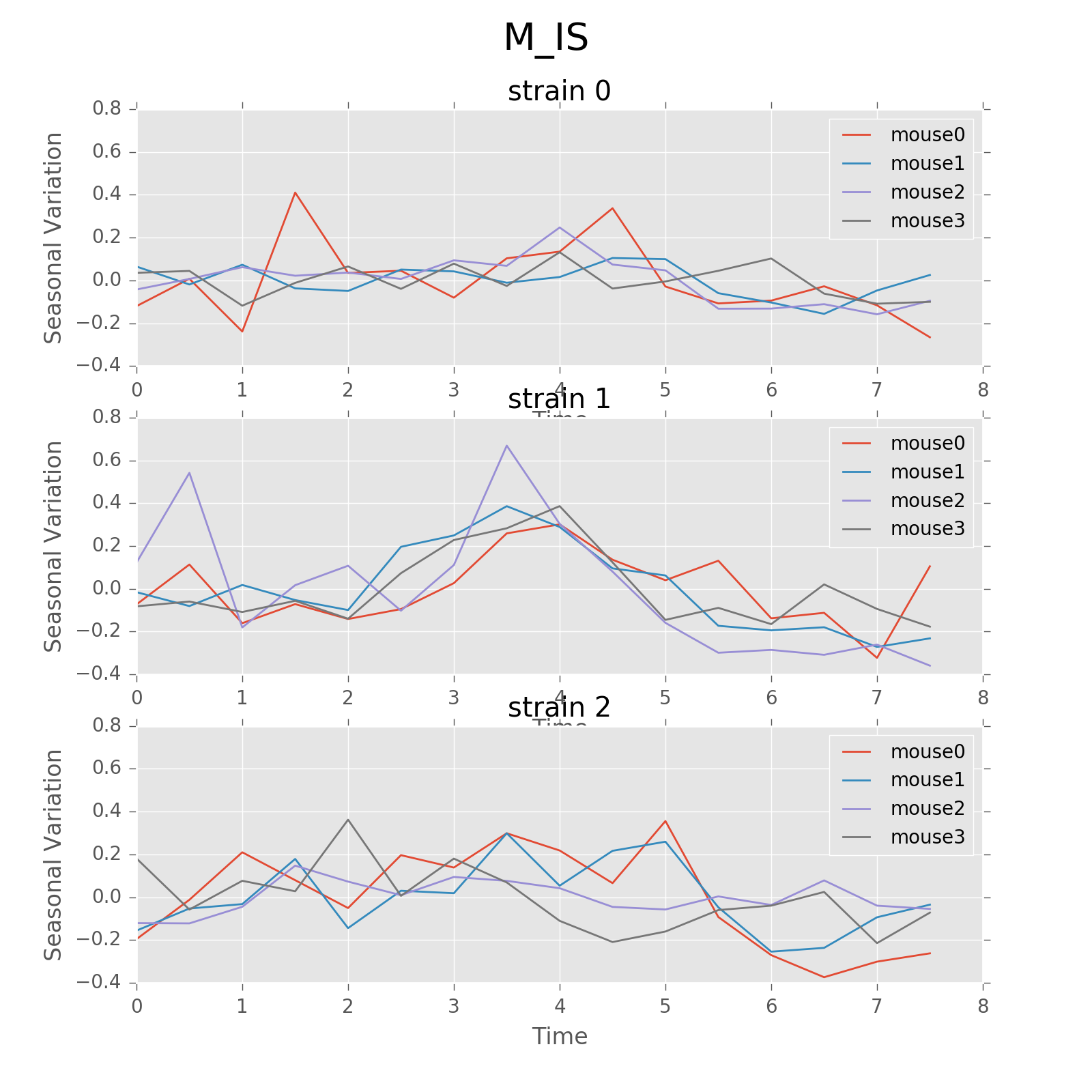
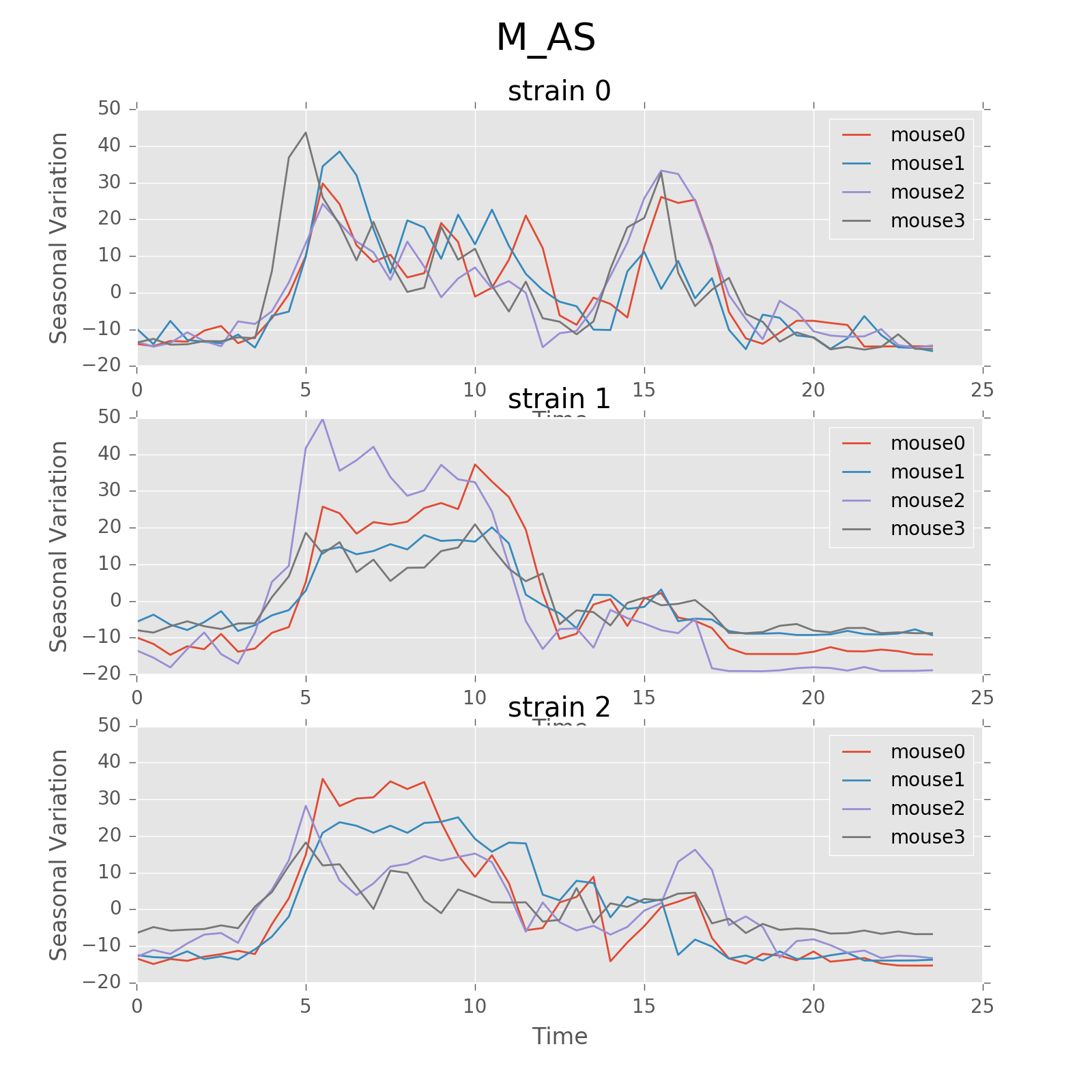
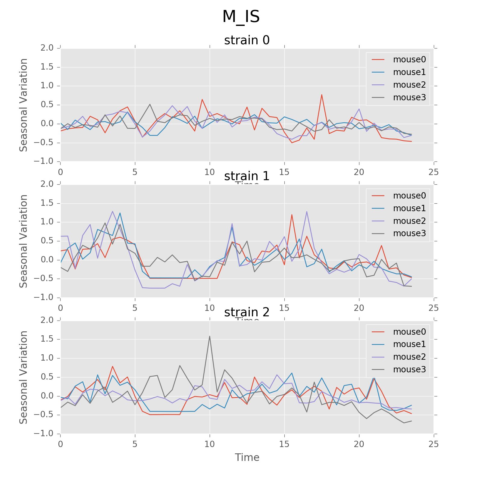
Below are the ultradian analysis results found by combining seasonal decomposition with best periods returned by Lomb Scargle periodogram. Here we use features “AS” (active state probability) and “M_IS” (movement time inside home base) as two examples, because other features like food, water, movement distance, movement time outside home base all have similar LS plot to “AS” and we show them in Appendix. “M_IS” shows a rather different pattern.
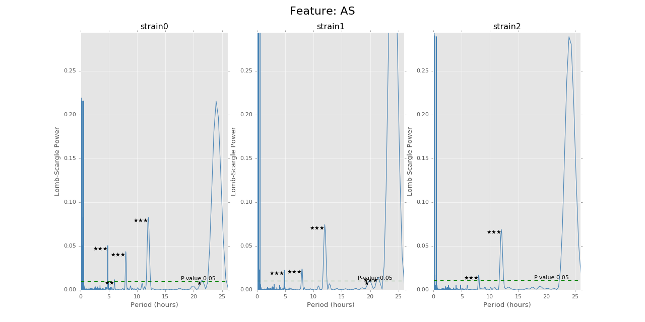
(png, hires.png, pdf) The ultradian analysis: seasonal decomposition using best periods returned by Lomb Scargle periodogram. For “AS” feature (active state probability), 12 hours is the common significant periods for all 3 strains (with p values smaller than 0.001). For “M_IS” feature (movement time inside home base), 8 hours appears to be the common significant periods for all 3 strains (with p values smaller than 0.01). There are certain kinds of consistent patterns within each strain. However, the signals are not as strong as in circadian ones (24 hours) shown in Seasonal decomposition and Appendix parts.

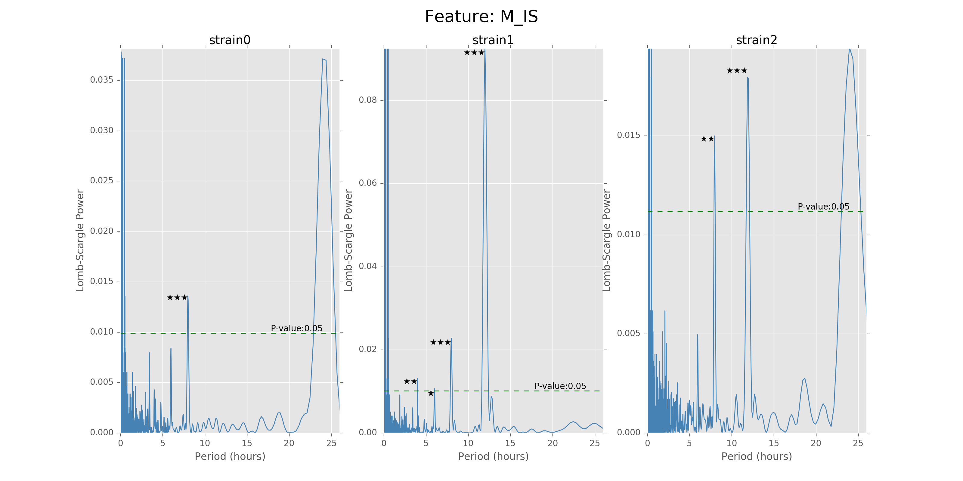
(png, hires.png, pdf) The ultradian analysis: seasonal decomposition using best periods returned by Lomb Scargle periodogram. For “AS” feature (active state probability), 12 hours is the common significant periods for all 3 strains (with p values smaller than 0.001). For “M_IS” feature (movement time inside home base), 8 hours appears to be the common significant periods for all 3 strains (with p values smaller than 0.01). There are certain kinds of consistent patterns within each strain. However, the signals are not as strong as in circadian ones (24 hours) shown in Seasonal decomposition and Appendix parts.
(png, hires.png, pdf) The ultradian analysis: seasonal decomposition using best periods returned by Lomb Scargle periodogram. For “AS” feature (active state probability), 12 hours is the common significant periods for all 3 strains (with p values smaller than 0.001). For “M_IS” feature (movement time inside home base), 8 hours appears to be the common significant periods for all 3 strains (with p values smaller than 0.01). There are certain kinds of consistent patterns within each strain. However, the signals are not as strong as in circadian ones (24 hours) shown in Seasonal decomposition and Appendix parts.

(png, hires.png, pdf) The ultradian analysis: seasonal decomposition using best periods returned by Lomb Scargle periodogram. For “AS” feature (active state probability), 12 hours is the common significant periods for all 3 strains (with p values smaller than 0.001). For “M_IS” feature (movement time inside home base), 8 hours appears to be the common significant periods for all 3 strains (with p values smaller than 0.01). There are certain kinds of consistent patterns within each strain. However, the signals are not as strong as in circadian ones (24 hours) shown in Seasonal decomposition and Appendix parts.
Longitudinal data analysis
Attempts for mixed models
The mixed model is frequently used for longitudinal analysis. We should specify the random effects and fixed effects first. Since it is ultradian analysis, we only need to focus on the hour factor and their cycle which we can get from the previous LS test. The random effect is the mouse id. We have four different mice in one strain and only want to compare the different patterns among these three strains. So if we set the random effect to be mouse id, the effects from different mouses will be cancelled out and we can also test the significance of these effects. The response variable will be one of the six features listed before. After that we can use the mixed model to get the pattern of the movements in different time period.
Build the model
Take Food feature as an example. Here strain0 is a dummy variable indicating whether the mouse belongs to strain 0 or not and similarly for strain1. strain0hour and strain1hour indicate the interaction terms, which we add in order to figure out whether the strain and hour have some interaction effect in the Food feature.(i denote ith strain, j denote the jth mouse)
Perform significance test
Here we have two purposes. The first is to figure out if the effects from different mouses are significant. The second is to figure out if the patterns for different strains are significantly different. To test the first one, we just need to use the t-test and get the p-value from the result by using the statsmodels.formula.api package. package. For the second one, we can perform the likelihood ratio test on the interaction terms.
First, we look at the summary of the full model (also take the Food feature as an example). To get this result, we fit the second-degree function. Since the cycles from the previous study are very similar between strains, we did not include it here. We can see that the effects of the mouse from the same strain are not significant. However, the p-value here seems to indicate that the interaction terms is not as significant as the other factors. So we consider conducting the likelihood ratio test.
| factors | Coef. | Std.Err. | z | P>|z| |
|---|---|---|---|---|
| Intercept | 0.049 | 0.008 | 6.095 | 0.000 |
| hour | -0.005 | 0.001 | 14.961 | 0.000 |
| hour2 | -0.001 | 0.000 | -18.767 | 0.000 |
| strain0 | -0.027 | 0.010 | -2.624 | 0.009 |
| strain1 | 0.045 | 0.010 | 4.332 | 0.000 |
| strain0:hour | -0.002 | 0.002 | -0.778 | 0.437 |
| strain1:hour | -0.004 | 0.000 | -1.76 | 0.078 |
| strain0:hour2 | 0.000 | 0.000 | 2.019 | 0.043 |
| strain1:hour2 | 0.000 | 0.000 | 0.540 | 0.589 |
| RE | 0.000 | 0.000 |
Secondly we did likelihood ratio test between the two models: full model and reduced interaction terms model. We found that the p values for 6 features below:
| Water | Food | AS | M_AS | M_IS | Distance |
|---|---|---|---|---|---|
| 3.08e-9 | 2.50e-9 | 9.39e-12 | 5.11e-5 | 0.002 | 1.53e-8 |
We can see that the Water, Food, AS, M_AS, Distance have significantly different patterns of different strains.
Testing Framework Outline
Step 1: Generating random samples for testing:
- Split the data based on the Mouse Day Cycle
- Number the splits and use numpy.random to subset from these splits
Step 2: Conduct Lomb-Scargle (LS) test to detect the period. Implement the three different models onto the certain period and get the patterns/ estimated coefficients for the model.
Step 3: Compare the result with our hypothesis.
Appendix
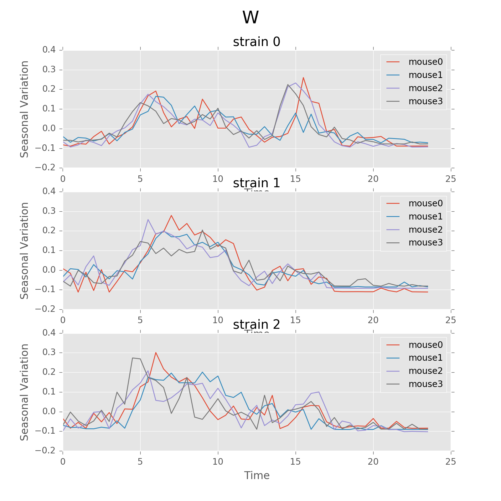
Seasonal variation of other features (circadian). Strain0 and strain1 have more obvious patterns than strain3, which is consistent with the findings in longitudinal data analysis.
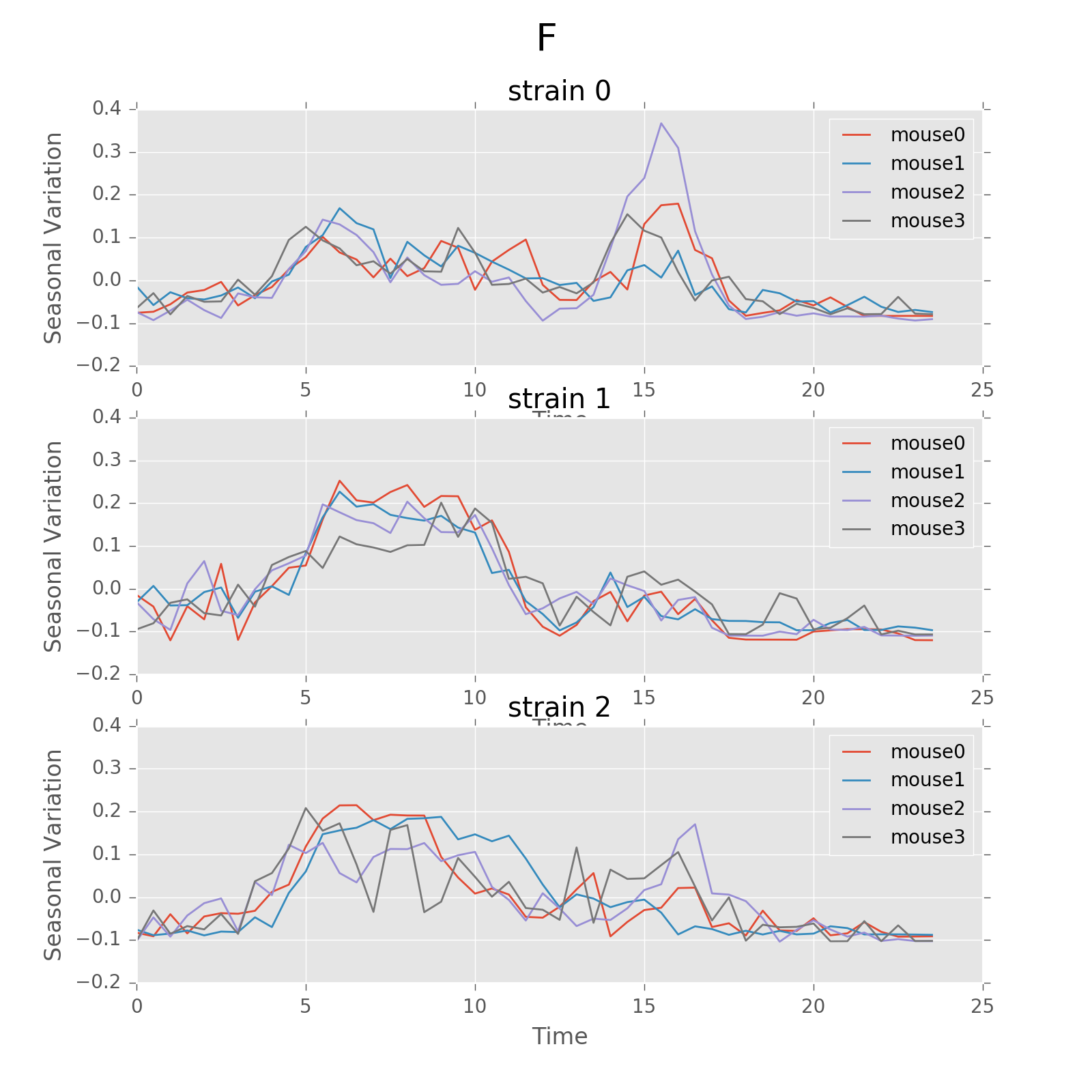
Seasonal variation of other features (circadian).
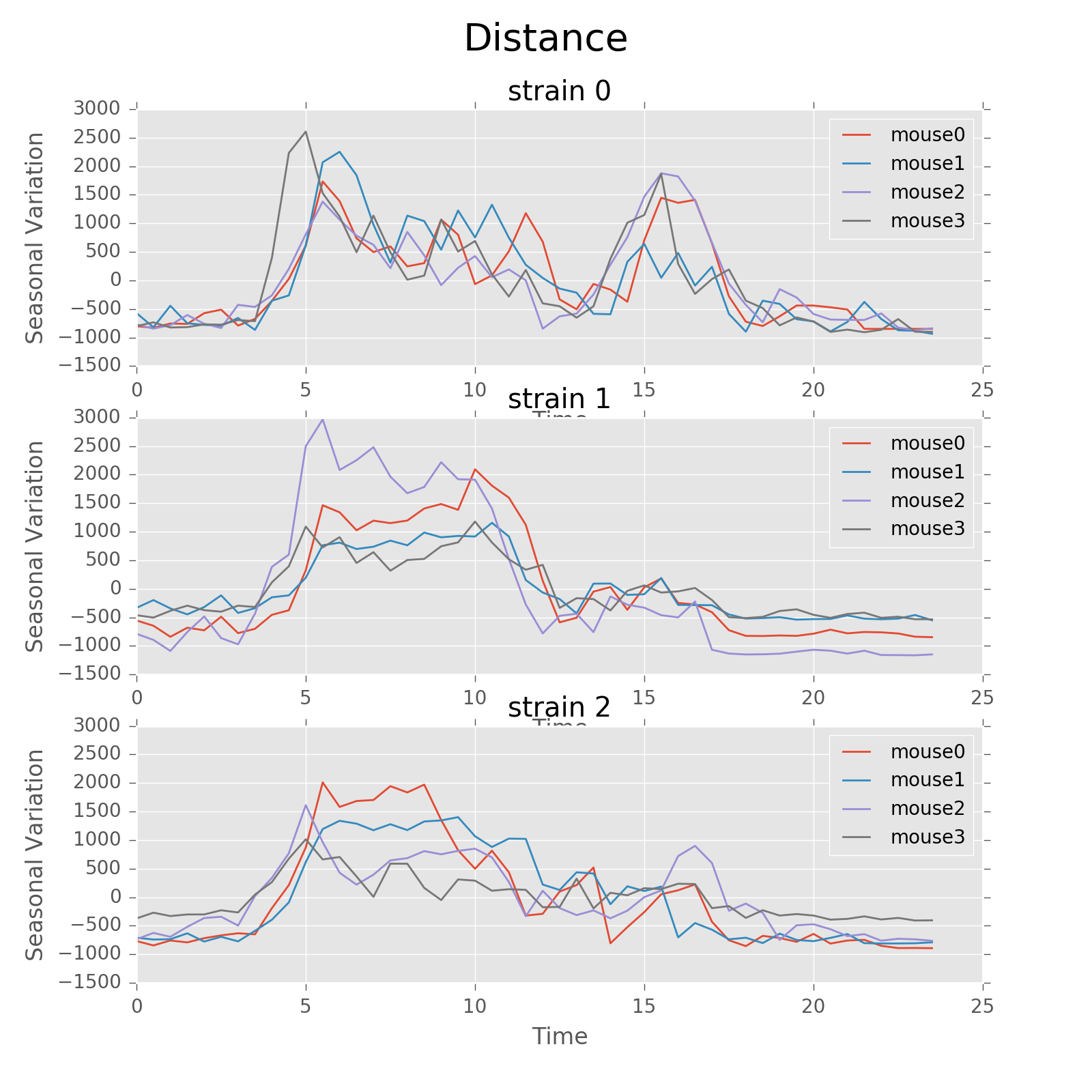
Seasonal variation of other features (circadian).
Seasonal variation of other features (circadian).
Seasonal variation of other features (circadian). Strain0 and strain1 have more obvious patterns than strain3, which is consistent with the findings in longitudinal data analysis.
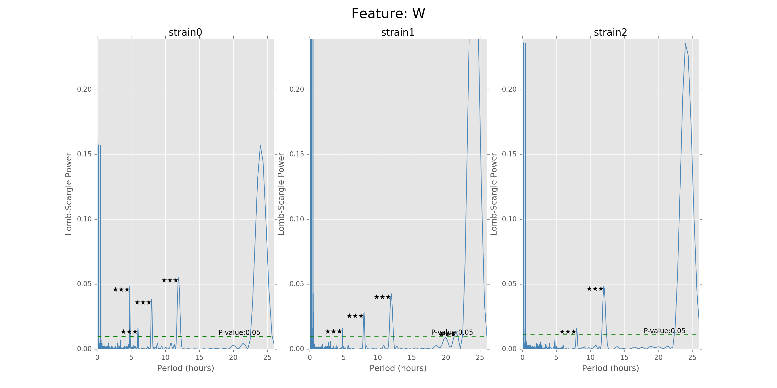
Lomb scargle plot for different features. Different strains have different ultradian periods, differing also in p-values. Here \(O(N\log N)\) algorithms suffer an instability around 0 points while \(O(N^2)\) algorithms can be more smooth. We here compare the significant ultradian periods between strains and ignore the highest LS power appearing near 24 hours.
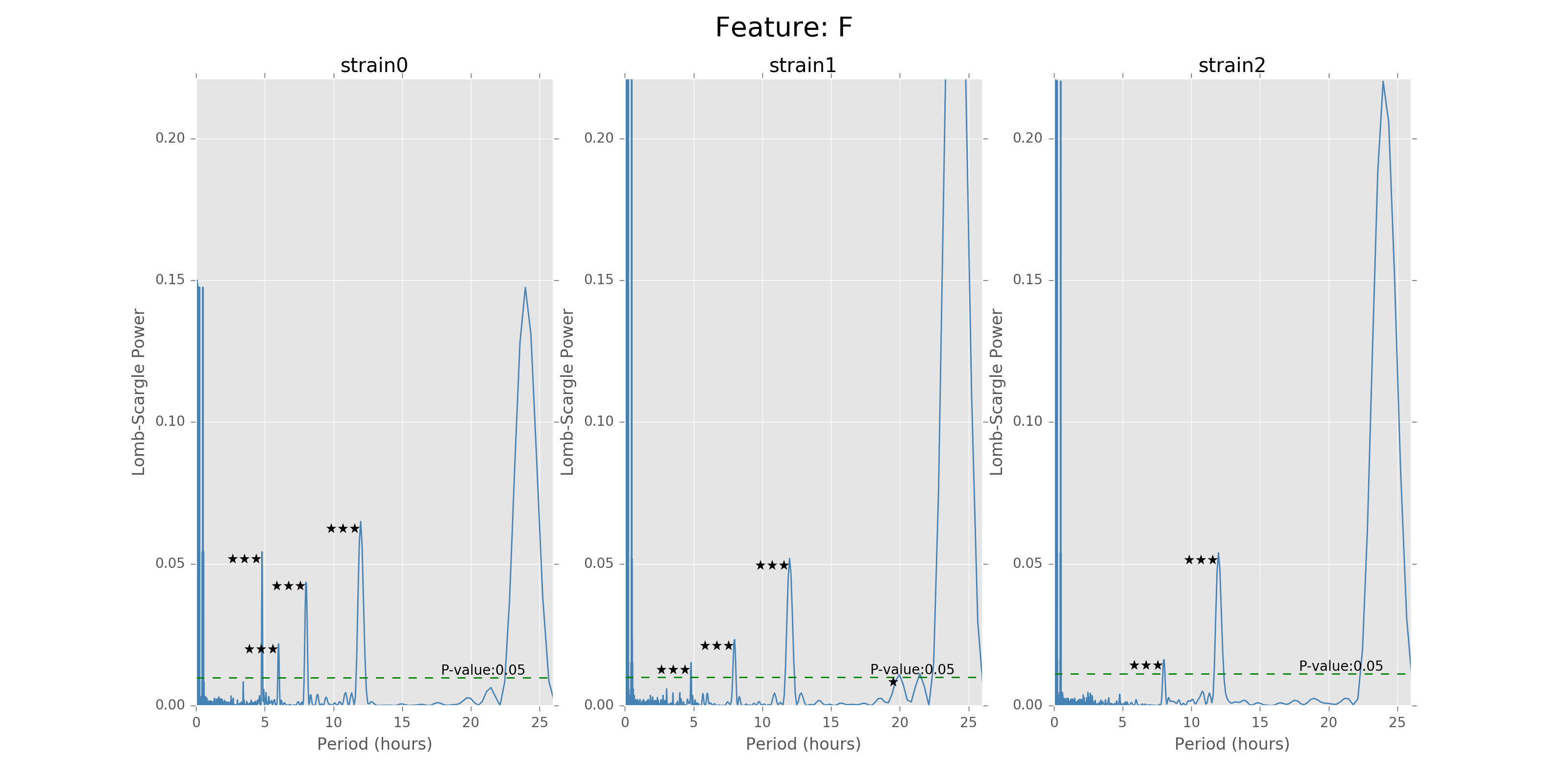
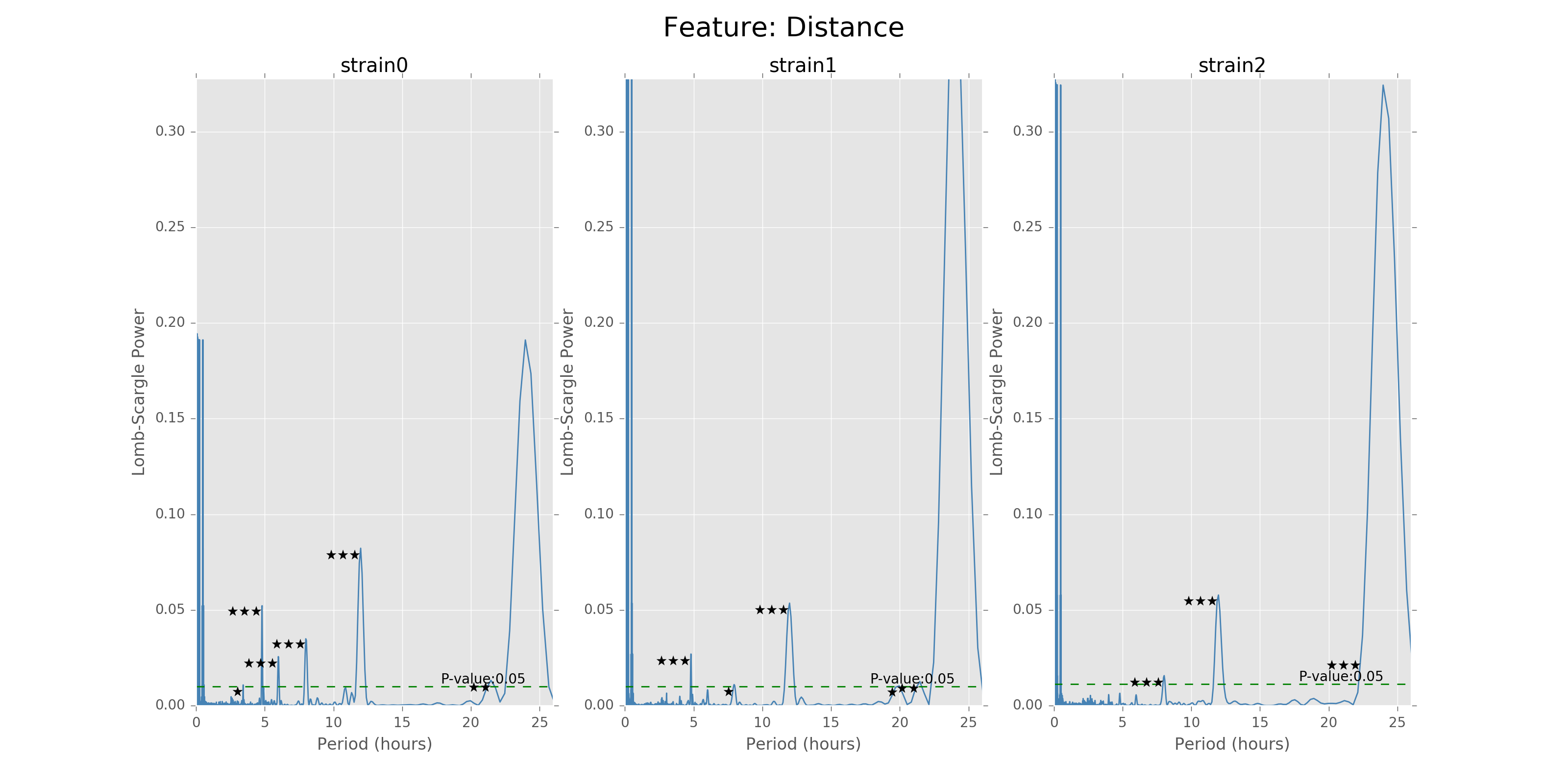


Lomb scargle plot for different features. Different strains have different ultradian periods, differing also in p-values. Here \(O(N\log N)\) algorithms suffer an instability around 0 points while \(O(N^2)\) algorithms can be more smooth. We here compare the significant ultradian periods between strains and ignore the highest LS power appearing near 24 hours.