Behavioral Model

Statement of Problem

In order to differentiate mice, we need to create a detailed behavior profile to describe:

1. how they drink, feed or move (locomotion) and
2. how they translate between active state or inactive state.

We have the following key background information from the paper:

• Home Cage Monitoring System(HCM) HCM cages were spatially

  discretized into a 12 x 24 array of cells and occupancy times for each MD were computed as the proportion of time spent within each of the 288 cells. To determine whether animals establish a Home base, HCM cages were spatially discretized into a 2 x 4 array of cells, and occupancy times for each mouse day were calculated as above. In the experiment, 56/158 animals displayed largest occupancy times in the cell containing the niche area, which was considered to be their Home base location.

• Active and Inactive State Mice react differently during

  Active state and Inactive states and all behavioral record should be classified into 2 mutually exclusive categories, Active States (ASs) and Inactive States (ISs). To designate ISs, we examined all time intervals occurring between movement, feeding, and drinking events while the animal was outside the Home base. Those time intervals exceeding an IS Threshold (IST) duration value were classified as ISs; the set of ASs was then defined as the complement of these ISs. Equivalent mathematically, ASs can also be defined as those intervals resulting from connecting gaps between events outside the Home base of length at most IST; ISs are then defined as the complement of these ASs. (Active State Organization of Spontaneous Behavior Patterns, C. Hillar et al.)

Statement of Statistical Problems

The above flowchart shows the key metrics that are required by the study to capture the behavioral profile:

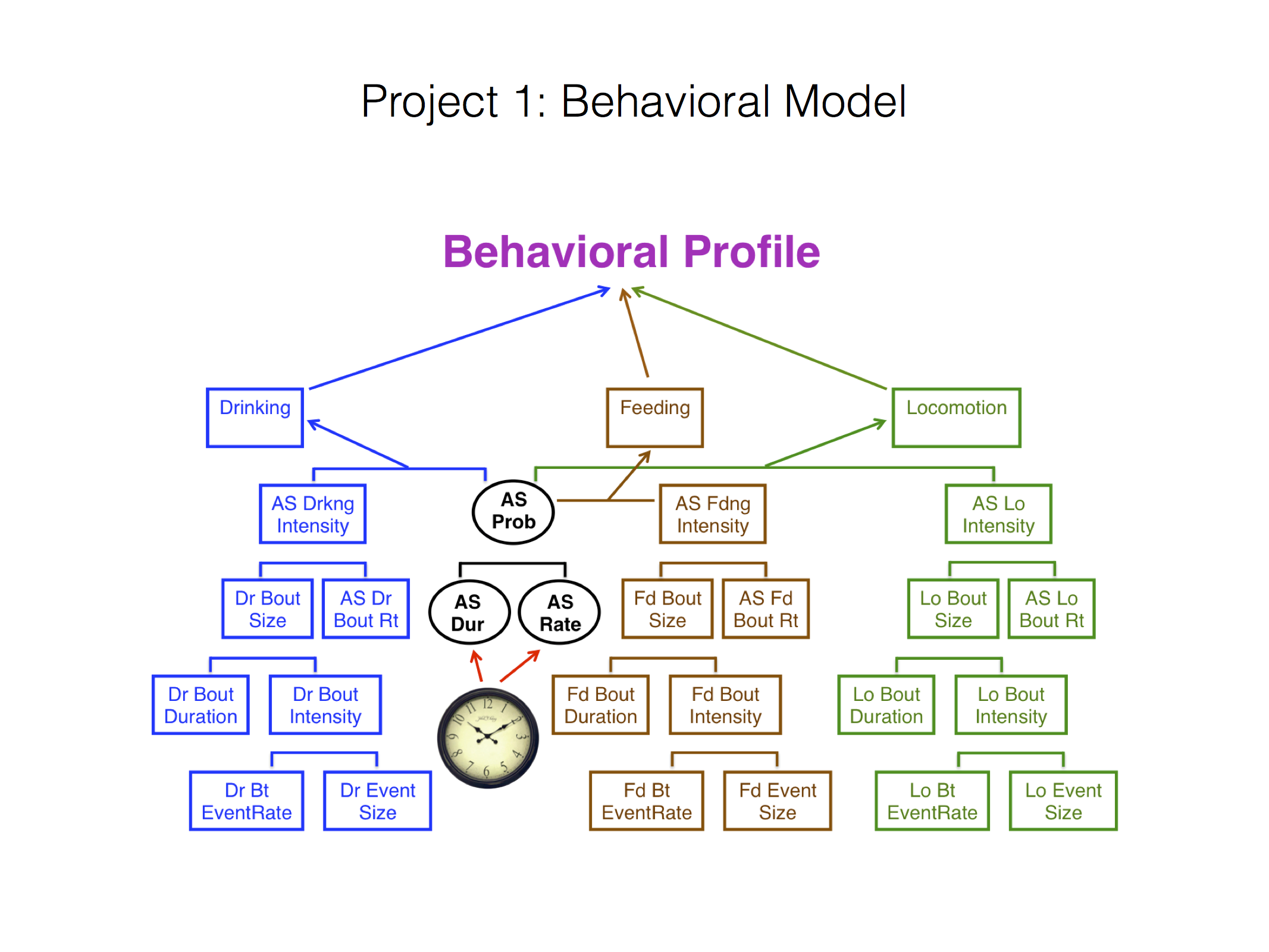
Behavioral Profile (image courtesy of Tecott Lab)

The main focus is 3 key states of the mice i.e. Drinking, Feeding and Locomotion.

Each of these metrics can be seen visually in the slides referenced below. Each metric is a tree, decomposed into two child node metrics, whereby when the child nodes are multiplied together, they yield the parent metric. We illustrate the relevant calculations in the case of drinking state:

Drinking Consumption Rate: Total Drinking Amount/ Total Time (mg/s)

Active State Prob: Active Time/ Total Time

Drinking Intensity: Total Drinking Amount/ Active Time (mg/s)

• Drinking Bout Rate: Number of Bouts/ Active Time (bouts/s)

• Drinking Bout Size: Total Drinking Amount/ Number of Bouts (mg/bout)

  • Drinking Bout Duration: Total Drinking Time/ Number of Bouts (s/bout)

  • Drinking Bout Intensity: Drinking Amount/ Total Drinking Time (mg/s)

    • Drinking Bout Event Rate: Number of Events/ Total Drinking Time (events/s)
    • Drinking Event Size: Total Drinking Amount/ Number of Events (mg/event)

Data

Our underlying functions depend on the following key data requirements for each mouse, strain and day:

• Active State
• Inactive State
• Moving Active State
• Moving Inactive State
• Total Distance Travelled (meters)
• Food Consumption (grams)
• Water Consumption (milligrams)

These data requirements are sourced via the mousestyles data loader utilities.

The Food and Water consumption data was only provided on a daily basis and our behavior utilities assume that such quantities are uniformly consumed over the time period studied.

Illustrative Examples

We illustrate the use of the behavior utilties with a motivating research question:

How do do the key feeding metrics compare across 2 different mice for the entire 11 days?

In this code, we see a few important features. First, we create behavior trees using the compute_tree function, and demonstrate their pretty-printing functionality. Then, we merge lists of trees into one larger tree of lists, which we can then summarize or turn into a Pandas data frame. Finally, we show how to plot the results using matplotlib.

#!/usr/bin/python

import mousestyles.behavior as bh
import numpy as np
import pandas as pd
import matplotlib.pyplot as plt

# get a tree for each day for two different mice
mouse1_trees = [bh.compute_tree('F', 0, 0, d) for d in range(11)]
mouse2_trees = [bh.compute_tree('F', 0, 1, d) for d in range(11)]
print(mouse1_trees[0])
print(mouse2_trees[0])

# merge each of the trees for the two mice
mouse1_merged = bh.BehaviorTree.merge(*mouse1_trees)
mouse2_merged = bh.BehaviorTree.merge(*mouse2_trees)
print(mouse1_merged)
print(mouse2_merged)

# get the means for the two mice
print(mouse1_merged.summarize(np.mean))
print(mouse2_merged.summarize(np.mean))

# turn the tree into pandas DataFrame
mouse1_df = pd.DataFrame.from_dict(mouse1_merged.contents)
# this gives us another way to compute summary statistics
print(mouse1_df.describe())


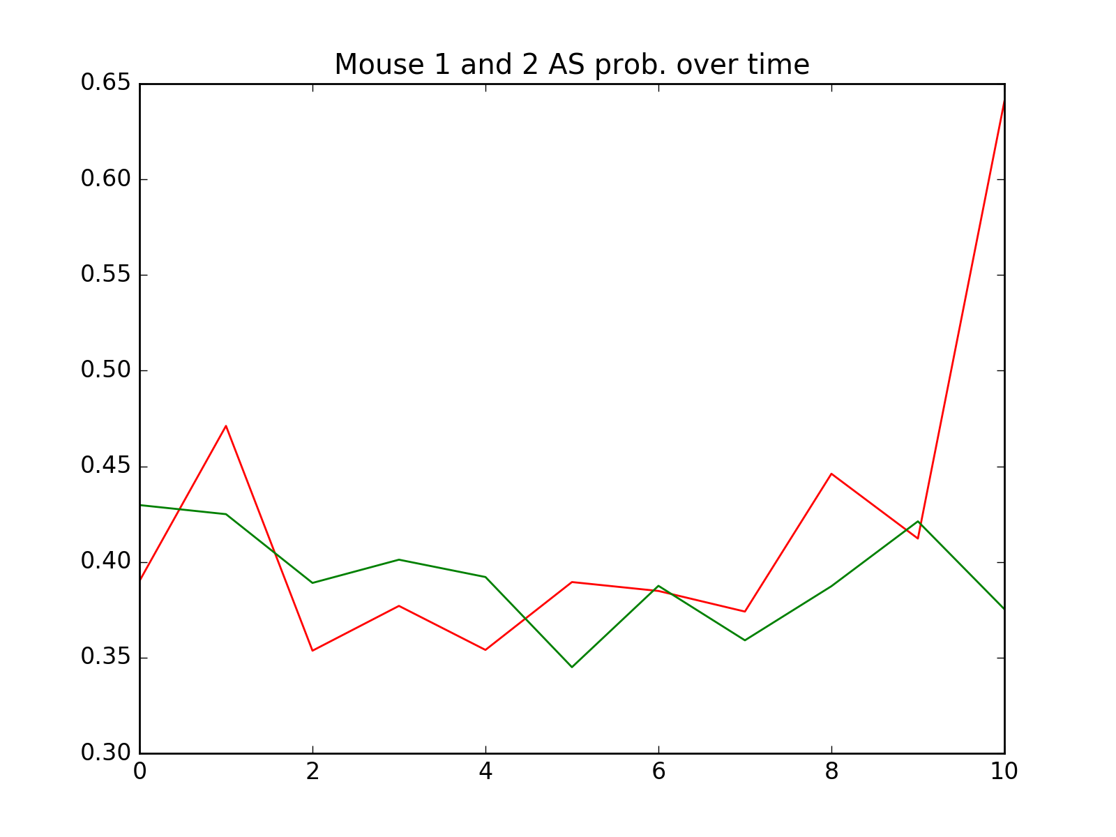
# plot the AS Probability over time
plt.plot(range(11),
         mouse1_merged['AS Prob'], 'r',
         mouse2_merged['AS Prob'], 'g')
plt.title('Mouse 1 and 2 AS prob. over time')
plt.show()

(Source code, png, hires.png, pdf)

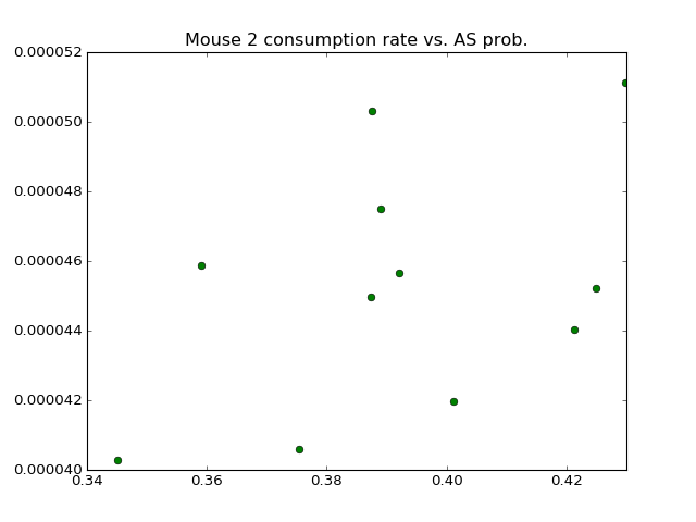
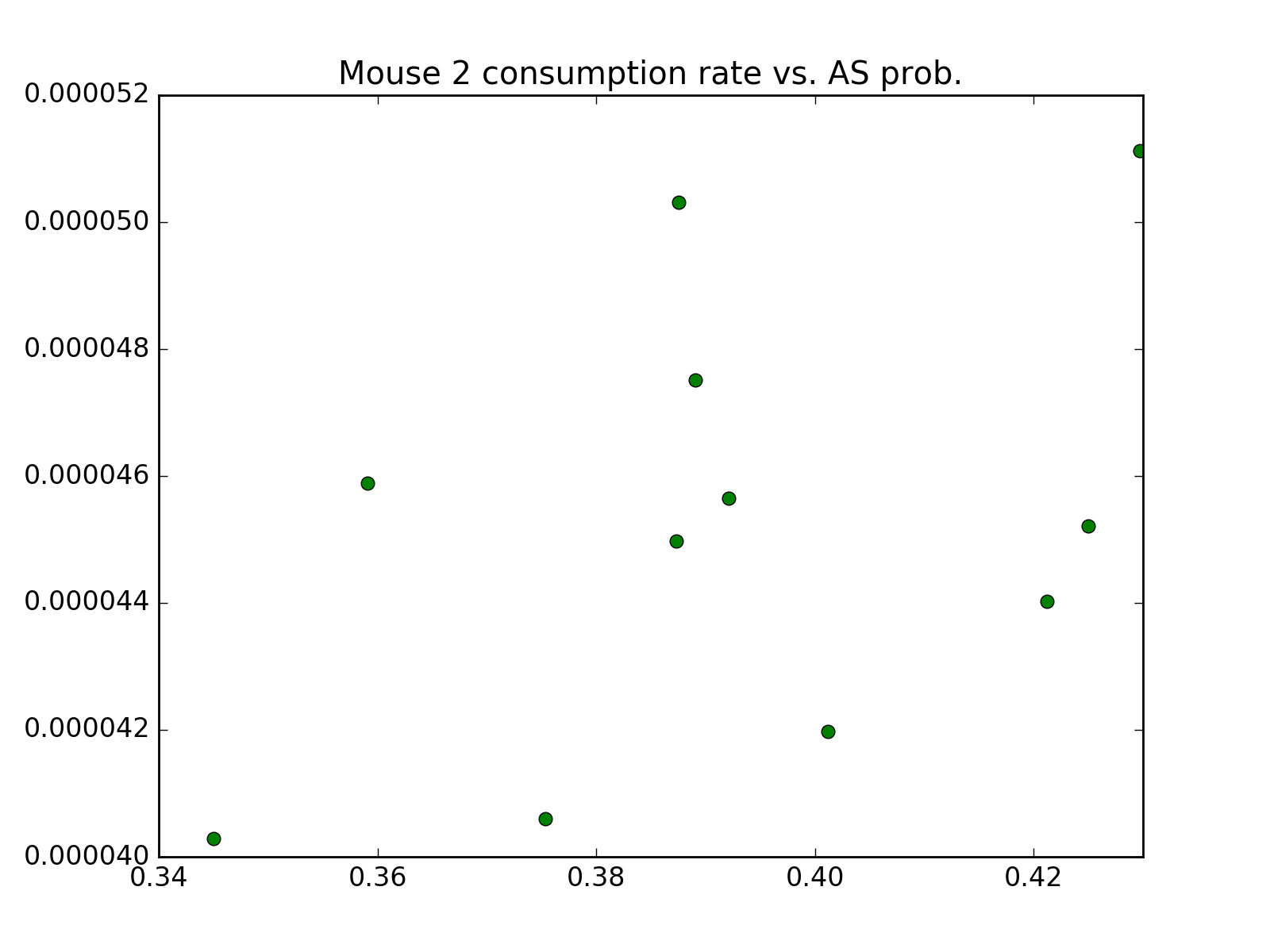
# plot consumption vs. AS prob
plt.plot(mouse2_merged['AS Prob'],
         mouse2_merged['Consumption Rate'], 'go')
plt.title('Mouse 2 consumption rate vs. AS prob.')
plt.show()

(png, hires.png, pdf)